Basic Concepts
Definition 1: We use the same terminology as in Definition 3 of Regression Analysis, except that the degrees of freedom dfRes and dfReg are modified to account for the number k of independent variables.
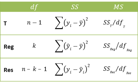
Property 1:
![]()
![]()
![]()
Proof: The proof is the same as for Property 1 of Regression Analysis.
Property 2: Where R is the multiple correlation coefficient (defined in Definition 1 of Multiple Correlation)
![]()
![]()
![]()
Proof: These properties are the multiple regression counterparts to Properties 2, 3 and 5f of Regression Analysis, respectively, and their proofs are similar.
Observation: From Property 2 and the second assertion of Property 3,
![]()
which is the multivariate version of Property 1 of Basic Concepts of Correlation.
Property 3: ![]()
Property 4: MSRes is an unbiased estimator of 
Observation: Based on Property 4 and Property 4 of Multiple Regression using Matrices, the covariance matrix of B can be estimated by
![]()
In particular, the diagonal of C = [cij] contains the variance of the bj, and so the standard error of bj can be expressed as
![]()
Example
Example 1: Calculate the linear regression coefficients and their standard errors for the data in Example 1 of Least Squares for Multiple Regression (repeated below in Figure using matrix techniques.

Figure 1 – Creating the regression line using matrix techniques
The result is displayed in Figure 1. Range E4:G14 contains the design matrix X and range I4:I14 contains Y. The matrix (XTX)-1 in range E17:G19 can be calculated using the array formula
=MINVERSE(MMULT(TRANSPOSE(E4:G14),E4:G14))
Per Property 1 of Multiple Regression using Matrices, the coefficient vector B (in range K4:K6) can be calculated using the array formula:
=MMULT(E17:G19,MMULT(TRANSPOSE(E4:G14),I4:I14))
H-hat
The predicted values of Y, i.e. Y-hat, can then be calculated using the array formula
=MMULT(E4:G14,K4:K6)
Standard Errors
The standard error of each of the coefficients in B can be calculated as follows. First calculate the array of error terms E (range O4:O14) using the array formula I4:I14 – M4:M14. Then just as in the simple regression case SSRes = DEVSQ(O4:O14) = 277.36, dfRes = n – k – 1 = 11 – 2 – 1 = 8 and MSRes = SSRes/dfRes = 34.67 (see Multiple Regression Analysis for more details).
By the Observation following Property 4 it follows that MSRes (XTX)-1 is the covariance matrix for the coefficients, and so the square root of the diagonal terms are the standard error of the coefficients. In particular, the standard error of the intercept b0 (in cell K9) is expressed by the formula =SQRT(I17), the standard error of the color coefficient b1 (in cell K10) is expressed by the formula =SQRT(J18), and the standard error of the quality coefficient b2 (in cell K11) is expressed by the formula =SQRT(K19).
Worksheet Functions
Excel Functions: The functions SLOPE, INTERCEPT, STEYX and FORECAST don’t work for multiple regression, but the functions TREND and LINEST do support multiple regression as does the Regression data analysis tool.
TREND works exactly as described in Method of Least Squares, except that the second parameter R2 will now contain data for all the independent variables.
LINEST works just as in the simple linear regression case, except that instead of using a 5 × 2 region for the output a 5 × k region is required where k = the number of independent variables + 1. Thus for a model with 3 independent variables you need to highlight an empty 5 × 4 region. As before, you need to manually add the appropriate labels for clarity.
Example 2: We revisit Example 1 of Multiple Correlation, analyzing the model in which the poverty rate can be estimated as a linear combination of the infant mortality rate, the percentage of the population that is white and the violent crime rate (per 100,000 people).
We need to find the parameters b0, b1 and such that
Poverty (predicted) = b0 + b1 ∙ Infant + b2 ∙ White + b3 ∙ Crime.
We illustrate how to use TREND and LINEST in Figure 2.

Figure 2 – TREND and LINEST for data in Example 1
Here we show the data for the first 15 of 50 states (columns A through E) and the percentage of poverty forecasted when infant mortality, percentage of whites in the population and crime rate are as indicated (range G6:J8). Highlighting the range J6:J8, we enter the array formula =TREND(B4:B53,C4:E53,G6:I8). As we can see from Figure 2, the model predicts a poverty rate of 12.87% when infant mortality is 7.0, whites make up 80% of the population and violent crime is 400 per 100,000 people.
Figure 2 also shows the output from LINEST after we highlight the shaded range H13:K17 and enter =LINEST(B4:B53,C4:E53,TRUE,TRUE). The column headings b1, b2, b3 and intercept refer to the first two rows only (note the order of the coefficients). The remaining three rows have two values each, labeled on the left and the right.
Thus, we see that the regression line is
Poverty = 0.437 + 1.279 ∙ Infant Mortality + .0363 ∙ White + 0.00142 ∙ Crime
Here Poverty represents the predicted value. We also see that R Square is .337 (i.e. 33.7% of the variance in the poverty rate is explained by the model), the standard error of the estimate is 2.47, etc.
Data Analysis Tool
We can also use Excel’s Regression data analysis tool to produce the output in Figure 3. This tool works exactly as in the simple linear regression case (see Hypothesis Testing Regression Slope), except that additional charts are produced for each of the independent variables.

Figure 3 – Output from Regression data analysis tool
Since the p-value = 0.00026 < .05 = α, we conclude that the regression model is a significantly good fit; i.e. there is only a 0.026% possibility of getting a correlation this high (.58) assuming that the null hypothesis is true.
Note that the p-values for all the coefficients with the exception of the coefficient for infant mortality are bigger than .05. This means that we cannot reject the hypothesis that they are zero (and so can be eliminated from the model). This is also confirmed from the fact that 0 lies in the interval between the lower 95% and upper 95% (i.e. the 95% confidence interval) for each of these coefficients.
Reduced model
If we rerun the Regression data analysis tool only using the infant mortality variable we get the results shown in Figure 4.

Figure 4 – Reduced regression model for Example 1
Once again we see that the model Poverty = 4.27 + 1.23 ∙ Infant Mortality is a good fit for the data (p-value = 1.96E-05 < .05). We also see that both coefficients are significant. Most importantly we see that R Square is 31.9%, which is not much smaller than the R Square value of 33.7% that we obtained from the larger model (in Figure 3). All of this indicates that the White and Crime variables are not contributing much to the model and can be dropped.
See Testing the Significance of Extra Variables on the Regression Model for more information about how to test whether independent variables can be eliminated from the model.
Click here to see an alternative way of determining whether the regression model is a good fit.
Complete Analysis Tool Output
Example 3: Determine whether the regression model for the data in Example 1 is a good fit using the Regression data analysis tool.
The results of the analysis are displayed in Figure 5.

Figure 5 – Output from the Regression data analysis tool
Since the p-value = 0.00497 < .05, we reject the null hypothesis and conclude that the regression model of Price = 1.75 + 4.90 ∙ Color + 3.76 ∙ Quality is a good fit for the data. Note that all the coefficients are significant. That R square = .85 indicates that a good deal of the variability of Price is captured by the model.
Observation: We can calculate all the entries in the Regression data analysis in Figure 5 using Excel formulas as follows:
Regression Statistics
- Multiple R – SQRT(F7) or calculate from Definition 1 of Multiple Correlation
- R Square = G14/G16
- Adjusted R Square – calculate from R Square using Definition 2 of Multiple Correlation
- Standard Error = SQRT(H15)
- Observations = COUNT(A4:A14)
ANOVA
- SST = DEVSQ(C4:C14)
- SSReg = DEVSQ(M4:M14) from Figure 3 of Method of Least Squares for Multiple Regression
- SSRes = G16-G14
- All the other entries can be calculated in a manner similar to how we calculated the ANOVA values for Example 1 of Testing the Fit of the Regression Line (see Figure 1 on that webpage).
Coefficients (in the third table)
We show how to calculate the intercept fields; the color and quality fields are similar.
- The coefficient and standard error can be calculated as in Figure 3 of Method of Least Squares for Multiple Regression
- t Stat = F19/G19
- P-value = T.DIST.2T(ABS(H19),F15)
- Lower 95% = F19-T.INV.2T(0.05,F15)*G19
- Upper 95% = F19+T.INV.2T(0.05,F15)*G19
The remaining output from the Regression data analysis is shown in Figure 6.

Figure 6 – Residuals/percentile output from Regression
Residual Output
Observations 1 through 11 correspond to the raw data in A4:C14 (from Figure 5). In particular, the entries for Observation 1 can be calculated as follows:
- Predicted Price =F19+A4*F20+B4*F21 (from Figure 5)
- Residuals =C4-F26
- Std Residuals =G26/STDEV.S(G26:G36)
Probability Output
- Percentile: cell J26 contains the formula =100/(2*E36), cell J27 contains the formula =J26+100/E36 (and similarly for cells J28 through J36)
- Price: these are simply the price values in the range C4:C14 (from Figure 5) in sorted order. E.g. the Real Statistics array formula =QSORT(C4:C14) can be placed in range K26:K36.
Finally, the data analysis tool produces the following scatter diagrams.
Normal Probability Plot
- This plots the Percentile vs. Price from the table output in Figure 6. This plot is used to determine whether the data fits a normal distribution. It can be helpful to add the trend line to see whether the data fits a straight line. This is done by clicking on the plot and selecting Layout > Analysis|Trendline and choosing Linear Trendline.
- It plays the same role as the QQ plot. In fact except for the scale it generates the same plot as the QQ plot generated by the supplemental data analysis tool (switching the axes).

Figure 7 – Normal Probability Plot
The plot in Figure 7 shows that the data is a reasonable fit with the normal assumption.
Residual Plots
- One plot is generated for each independent variable. For Example 2, two plots are generated: Color vs. Residuals and Quality vs. Residuals.
- These plots are used to determine whether the data fits the linearity and homogeneity of variance assumptions. For the homogeneity of variance assumption to be met each plot should show a random pattern of points. If a definitive shape of dots emerges or if the vertical spread of points is not constant over similar length horizontal intervals, then this indicates that the homogeneity of variances assumption is violated.
- For the linearity assumption to be met the residuals should have a mean of 0, which is indicated by an approximately equal spread of dots above and below the x-axis.

Figure 8 – Residual Plots
The Color Residual plot in Figure 8 shows a reasonable fit with the linearity and homogeneity of variance assumptions. The Quality Residual plot is a little less definitive, but for so few sample points it is not a bad fit.
The two plots in Figure 9 show clear problems. Fortunately, these are not based on the data in Example 3.

Figure 9 – Residual Plots showing violation of assumptions
For the chart on the left of Figure 9 the vertical spread of dots on the right side of the chart is larger than on the left. This is a clear indication that the variances are not homogeneous. For the chart on the right the dots don’t seem to be random and also few of the points are below the x-axis (which indicates a violation of linearity). The chart in Figure 10 is ideally what we are looking for: a random spread of dots, with an equal number above and below the x-axis.

Figure 10 – Residuals and linearity and variance assumptions
Line Fit Plots
- One plot is generated for each independent variable. For Example 3, two plots are generated: one for Color and one for Quality. For each chart the observed y values (Price) and predicted y values are plotted against the observed values of the independent variable.

Figure 11 – Line fit plots for Example 3
Reporting Results
The results from Example 3 can be reported as follows:
Multiple regression analysis was used to test whether certain characteristics significantly predicted the price of diamonds. The results of the regression indicated the two predictors explained 81.3% of the variance (R2=.85, F(2,8)=22.79, p<.0005). It was found that color significantly predicted price (β = 4.90, p<.005), as did quality (β = 3.76, p<.002).
You could express the p-values in other ways and you could also add the regression equation: price = 1.75 + 4.90*color + 3.76*quality.
Examples Workbook
Click here to download the Excel workbook with the examples described on this webpage.
References
Microsoft (2014) LINEST function
https://support.microsoft.com/en-us/office/linest-function-84d7d0d9-6e50-4101-977a-fa7abf772b6d
Excel Easy (2025) Regression analysis in Excel
https://www.excel-easy.com/examples/regression.html#google_vignette
Hi Charles,
I am using this software to simulate the curve fitting, y=y0+Aexp(-x/t) which is namely ExpDec1 in Originlab software. Since there is only one independent parameter x in this equation, could this fitting belongs to multiple regression or linear regression? It is a curve, not line. Could you suggest the method to simulate such curve fitting based on Real Statistics Resource Pack? Actually, I have finished the nonlinear fitting using Originlab software, but I wish using Real Statistics Resource Pack and give a better understanding on the whole process. In addition, Could you explain the defference between the term multiple regression with curve fitting with a excel example?
Many thanks for your kindness and help.
yidong on Dec. 22, 2023
Hi Yidong,
1. Since you have only one independent variable, this is an example of regression, but not linear regression since it isn’t linear. Linear regression is of the form y = c + bx. With exp() in the equation you lose the linearity. You can use linear regression to get an approximate solution as described in
https://real-statistics.com/regression/exponential-regression-models/
2. You can also create a nonlinear regression model as described in
https://real-statistics.com/regression/exponential-regression-models/real-statistics-exponential-regression-functions/
This model will have a a little better fit to most data.
3. If you have more than one independent variable, then you would have multiple regression. If the resulting equation is linear (e.g y = ax1 + bx2 + c) then you would have multiple linear regression.
Charles
Hi charles,
I am looking for your help in knowing whether we can create multiple linear regression scatterplot output in excel like we do for simple linear regression .
If yes, please share the steps and oblige me .
Regards,
Hanspal
Business Statistic learner
Hi Hanspal,
It looks like you want a scatterplot in more than 2 dimensions. Excel has limited support for 3D plots. The Real Statistics software doesn’t provide support for multiple linear regression scatterplots.
Charles
TDIST and TINV have been updated. So
P-value=TDIST(ABS(H19),F15,2) should be T.DIST.2T(ABS(H19),F15)
and
Lower/Upper 95% should be F19-T.INV.2T(0.05,F15)*G19
*I accidentally posted this comment in the Multiple Correlation page. Sorry
Yes, you are correct. I have just updated the webpage to use the updated functions.
I am in the process of updating all the webpages to use the latest versions of the Excel worksheet functions.
Charles
Charles,
What you offer on these pages is heroic!
I hesitatingly ask: are the manually-entered coefficient labels in Figure 2 in the wrong order: b1, b2, b3; when they should be b3, b2, b1?
I’ve been puzzling through how to set up a VAR(n) in Excel, with something like 5 variables and 12 lags (a la a recent Vanguard article on forecasting CAPEs). I think I saw that maybe someday you’ll have some capability available. That would be great because this seems like a very messy thing to organize and run in Excel (or even VBA).
Thank you again for all your efforts and insights!
Blake
Blake,
1. Yes, you are correct. The order of the coefficients in the figure is not correct. I have now corrected the image on the webpage. Thank you for finding this error.
2. I don’t know what you are referring to re VAR(n). Can you give me a reference?
Charles
Thank you Charles,
Sorry, I was referring to a Vector AutoRegressive (VAR) model, for example, with a lag of 12 and five variables:
Xt= α+ β1Xt−1+ β2Xt−2+⋯+ β12Xt−12+εt,
where 𝑿𝑡 is a vector of the five variables in the VAR model.
As I mentioned, I thought you indicated somewhere that someday you might do something in this area.
Also, I’ve recently also been working on “Partial Sample Regression,” which looks like a very valuable new tool in the regression realm. You may want to take a look sometime (see the attached example paper).
Thanks again and my best wishes!
Blake
Blake,
Thanks for your suggestions. I looked at the paper you referenced about Partial Sample Regression and it looks interesting. I will add both items to the list of possible future enhancements (actually VAR is already on the list). Thanks again and Happy New Year.
Charles
Dear Charles,
thank you for your help again. Now, it works and gives me results. The complexity now is to understand them and best use the tool. But this is my problem.
All the best
Fritz
Fritz,
That is good to hear.
Charles
Dear Charles,
let me first thank you for your help and advice. I have downloaded your new release (my contact to you and to your packages is also new) and I have tried to use your function BRegCoeff to my problem and to an artificial test case but I did not succeed. The only output I got is one number, the intercept value. What do I possibly do wrong and is there somewhere an example for the use of BRegCoeff.
Thank you once more
Fritz
Dear Charles,
My problem consists of one dependent and 3 independent variables. The regression should be y=a1x1+a2x2+a3x3. I have 15 data sets. As it is a physics problem, a1 has to be positive and the other two negative. When I do the regression between y and xi separately for each xi, then indeed the signs come out correctly, a1 is positive, the others are negative. But the p-value is significant only for a1x1. When I do the regression both with x2 and x3, then both coefficients turn out negative as expected. When I select x1 and x2 then both coefficients are suddenly positive and this is nonsense in case of a2. The same is the case with the complete regression, y versus x1, x2 and x3. All ai are positive. Now I am lost with the interpretation. Maybe, you know what is wrong with my approach.
Thank you very much.
Fritz
Dear Charles,
I have acquired new data to refine a model M=A+3D-2.73 by means of a multiple regression analysis. The challenge is that the coefficient of A is fixed to 1 by definition. Is it possible to perform a multiple regression analysis for this case?
Martin,
Assuming that D is an independent variable and M is a dependent variable, with 3, and A-2.73 as constants, I don’t see any regression coefficients.
Charles
Charles,
What I mean is that M=aA+bD+c with M the dependent variable and A and D independent variables. I would like to determine regression coefficients a, b and c by means of a multiple regression analysis with new data I recently acquired.
What is known already is that (1) a previous analysis with old data found that b=3 and c=-2.73 so I expect my analysis to yield similar answers; (2) that a=1 per definition (this has never been questioned before as far as I know).
How to perform a multiple regression analysis for such a case?
What I am thinking is to define a new dependent variable MA=M-A=bD+c to solve b and c. But how would that influence the significance of goodness-of-fit and p-value of b? Especially since in a multiple regression (for a, b and c) coefficient a might turn out not be 1 but (I am guessing now) say 0.97? Is there a way to estimate that if (say for example) a=0.97 (and a is not equals 1) that this is close enough to a=1 that we can accept the goodness-of-fit and p-value for b as accurate enough for a credible result even if it was derived with the regression MA=M-A=bD+c?
Martin,
Yes, the regression equation takes the form MA = bD + c where MA = M-A. Thus, if for one data element M = 5, A = 3 and D = -3, you would use the pair MA = 2 and D = -3. You can then predict the values of MA based on the value of D. If you also know the value of A then you would then be able to predict the value of M.
Charles
Charles,
I have a set of 16 independent variables (df=16, n=40) that I am applying to 18 different sets of dependent variables. In the past, I have manually run the Data Analysis Tool Pack Regression on each set of dependents to get my coefficients for forecasting. However, I have recently started using LINEST to get the coefficients. Is there a new companion function in Excel to get the p-values that would have been in the Summary Output for each Regression run?
On top of all that, my independent variables change! So having a “function” based p-value calculation would be vastly superior to relying on a manually-run Tool Pack output. LINEST has already made a big impact on getting the coefficients quickly. Now I just need a function for p-value.
Really hoping you have a solution and I have just missed it. Appreciate all that you post here.
Thank you,
Micheal
Micheal,
You can use the Real Statistics software for this purpose. E.g. the RegTest function will output the p-value in Excel. You can download the software for free from
https://real-statistics.com/free-download/real-statistics-resource-pack/
Charles
Charles,
I have finally gotten around to this stage of my project. I’ve got Real Statistics up and running. Impressive. How did I not know about this all these years! Your selfless gift is remarkable.
Followup…
Just as you described, I can now use the RegTest function to get the p-value for the entire regression. But, I realize now I should have been more specific in my original question…
Better stated question…
Is there a single function that will provide the individual p-values for each independent variable?
At present, with some backwards engineering, I have used the RegCoeff function to get the coefficient, standard error, and then manually calculated the t statistic and finally p-values (via the 2T T distribution function). This produces an array of calculations that is accurate, but not optimal (structure).
I hope I am not off in the weeds, but my need for a single function is driven by data structuring. A single function for independent-variable-level p-values will allow me to keep certain arrays neatly organized (if that makes sense). I am trying to have a single column with an array of coefficients (LINEST) with an array of corresponding p-values just below the coefficients. This is because I am regressing the same set of Xs to different sets of Ys and desire to have these figures in the corresponding column of the Ys.
Sincerely,
Micheal
Michael,
Thanks for the clarification. Should the output from the function look like the following?
variable coeff— std err- t stat– p-value
Intercept 38.11916815 8.130254514 4.688557792 0.042604514
x1-Variable 0.069007609 0.300032424 0.230000504 0.839474192
x2-Variable 1.601933767 0.190142609 8.424906822 0.013797751
Charles
Sir,
How can we solve second order polynomial regression(multiple variables)equations? I have 3 variables(x,y&z) and considered the square terms(x^2,y^2,z^2) and (xy,yz and zx )terms along with (x,y,z) for analysis. I am not getting correct results from the matrix approach. Kindly help me out.
Anne,
See https://real-statistics.com/multiple-regression/polynomial-regression/
https://real-statistics.com/multiple-regression/interaction/
Charles
Thank you Sir
hi! can i ask how would i determine if my independent variables has an impact on the dependent variable?
Regression Statistics
R Square 0.20457801374462
Standard Error 9.16964563317025
Significance F
0.031673864
significance F is 0.0000626432618907069
This value is different from the one in your other comment, however, the conclusion is the same.
Charles
Since p-value = .031674864 < .05, generally this would be considered to be a significant result, yielding evidence that the independent variables have a significant impact on the dependent variable. Charles
How would I determine the impact of the indpenent variables on the depentdent variables? For example, the $ impact of unemployment, population, GDP on taxes revenues?
Hello Matt,
It depends on what you mean by “impact”, but the value of the regression coefficient for any particular independent variable tells the amount that the dependent variable increases for every increase of one unit of the independent variable.
Charles
I ran a model and found the following values. I know the model fits well, but don’t know what to make of the coefficients. All fo the p-values for the coefficients are <.05. What should I make of this? That the model is reliant on every coefficient? Or that there isn't one coefficient that is important?
Regression Statistics
R Square 0.732284957
Standard Error 0.078073613
Significance F
0.031673864
Taylor,
This means that all of the coefficients are significant (relevant).
Charles
Good day Charles!
I am doing a regression of a dependent variable which have three categories and a categorical independent variable. what do I do?
Thanks!
Hello Shine,
For the categorical independent variable, you need to use dummy coding. This is explained at
https://real-statistics.com/multiple-regression/multiple-regression-analysis/categorical-coding-regression/
Since you also have categories for the dependent variable, you should consider using logistic regression instead of linear regression. Since you have three categories you will need to use the multinomial version of logistic regression. See the following webpage for more details
Logistic Regression
Multinomial logistic regression
See the following webpage for how to create dummy codes for logistic regression using Real Statistics.
https://real-statistics.com/logistic-regression/handling-categorical-data/
One further remark: since both the independent and dependent variables are categorical, you may be able to use the chi-square test of independence (depending on why you want to do regression in the first place). See
Independence testing
Charles
I have four different data sets and want to plot them on the same graph. I want to show that the expression I have for the trend can be used accurately for all of them. How can I do this? Trend-wise its that same for all the plots on the graph and I have an expression already from excel trend lines. (ie I have an exponential trend)
Hello Ronald,
You can plot one data set and then add the exponential trend line. You then need to add each of the other three graphs to the same chart by clicking on the chart that you have created and choose Design > Data|Select Data. You then click on the Add button to add each of the other graphs. You can click on any of the points on the new graphs to add the trenline for that graph.
Charles
Dear Charles,
This I have already done but I still need to show that the equation is universal for all of them and that there is minimal error. My supervisor mentioned something like the use of least squares to show that the equation is universal for all the data sets.
If possible I could show you a photo of what I want to do.
Yes, you can show me a photo of what you want to do.
Hi there!
What I am looking for variable that discriminates another variable, how could I identify it based on the results? Please assist me on the plotting of results as well. Considering of the numerous results, identification of the data to be used / displayed is quite challenging for me. I hope you can assist me on this. Thank you.
Hi JM,
I am sorry but I don’t understand your comment. What do you mean by a variable that discriminates another variable?
Charles
Can you show the function string for the covar matrix in I17:K19, in Figure 1 above? I understand the logic but am having a hard time with constructing the function.
Brian,
=O19*E17:G19. This is an array function and so you must press the key sequence Ctrl-Shft-Enter
Charles
Brian,
=O19*E17:G19. This is an array function and so you must press the key sequence Ctrl-Shft-Enter
Charles
Hi Charles, the regression tool shows how much of the variance is being explained by the overall model via R2.
However, looking at the coefficients you refer to, I assume these are unstandardised regression coefficients or are they standardised? Or do they both show the importance of each variable relative to the other variables?
Also, how could I see the variance being explained by each IV? Or would I have to run a multiple regression again by excluding IVs – 1 at a time – to see how much each one contributes? With SPSS, I could square the part correlations from the output and so calculate semi-partial correlations (sri2).
Thanks Charles!
Demos,
The coefficients are for unstandardized regression. If you want standardized regression, see
Standardized Regression Coefficients
You can use the same approach that you described in SPSS. This is because Real Statistics will produce the exact same values as SPSS for the coefficients. You have another choice for determining the relative weights of the different independent variables on the regression model, namely using the Shapley-Owen Decomposition. See the following webpage:
Shapley-Owen Decomposition
Charles
Hi Charles, Hope you are well.
When running residual plots, I have seen variations of what is actually plotted. In your examples above, you run raw data of say color with the residuals.
When I looked at other residual plots from other websites, I have seen that Standardized predicted values and Standardized residuals were used. Is there any difference?
Demos.
Hi Charles,
I am running a few multiple regressions and have the summary outputs in a typical horizontal format like those summary outputs presented in your tutorial above. My problem, however, is that I am required to make my outputs in vertical format. I am using an original regression with an x^2 term in my Regression 1 and then following it up by adding interaction variables in my Regression 2 to show my Adj. R^2 increasing/SEE decreasing.
If you have any help on how I could make my outputs vertical to illustrate my change using interaction variables it would be much appreciated.
Matt
Matt,
You can do this manually, using formulas like =D5 to copy the relevant cells. Alternatively you can use the TRANSPOSE function to change rows to columns and columns to rows. Since the transpose function doesn’t handle formulas well, you might first need to copy the entire output from the regression analysis and paste as data (via File > Clipboard|Paste or Alt-HVV).
Charles
What a great tutorial! You are henceforward my first site to visit on any thorny question.
Thanks for your generous contribution to students everywhere. Bill Gates owes you $10 million. (Pocket change)
You keep an old retired Ph. D a little sharper in his declining years, too.
Dave,
Thank you very much for your kind words. You sussed me out completely.
I am glad that I can make my contribution and continue to learn things about mathematics and people all over the world.
Charles
Hello dear sir,
I am trying to make multiple regression analysis for data collected in likert scale. I have five independent variables and one dependent variable each having their own questions to be answered by respondents.I want to regress them in excel. could you please tell me the procedures i should go through to get the regression results?
Rahel,
This is explained on the referenced webpage. What additional information do you need?
Charles
Could you kindly provide the link to the webpage?
Aditya,
Which webpage are you referring to?
Charles
Hi Charles,
I am trying to calculate one beta for a multiple regression (1 dependent variable and 3 independent variables) and am not sure I am quite understanding what the best way to do this is?
If I use the LINEST function does this calculate the beta?
Or if I use the multiple regression analysis, is the first coefficient the beta for all variables or do I need to add up the 3 different coefficients to get the total beta?
Thanks,
Kiran
Kiran,
You can use LINEST or the multiple regression data analysis tool. In either case, all the beta coefficients are output. There is no total beta –it doesn’t exist and has no meaning.
Charles
Hello.
Sir, I need manual calculation in multiple regression for 6 independent variable using Ordinary Least Square. Is there exist tutorial for that ??
thank you for your goodness.
Bayu,
If you follow the approach described on the website you will be able to manually calculate multiple regression for 6 independent variables. See especially Multiple Regression using Matrices.
Charles
Hi Charles,
I have a question about interpreting the data.
In the examples you gave the variables that have a low p Value for the t-test are considered to have good predictive value for the final outcome. However in each of your examples the intercept had a very high P value.
Is there are any particular significance to this or is it a statistical artifact?
Jonathan,
It just means that the intercept is not significantly different from zero.
Charles
Hello Charles,
Thanks a lot. Just a suggestion: it seems that in the ‘Regression Statistics’, Standard Error = SQRT(H15) and not SQRT(H14).
Best regards,
Roland
Hello Roland,
Thanks for catching this typo. I have now corrected the formula on the referenced webpage. I appreciate your help in making the website more accurate and so easier to understand.
Charles
Hey Charles
I’m a medical doctor from Brazil and for some time now i use your exel tables on my scientific research. However i’m in a pinch.
To make things simple, the intercept value on the table that is created from a multi regression, what does it meanAnd its p value?
Vitor,
Excel’s Regression data analysis tool reports the intercept coefficient and its p-value. These are also reported using the Real Statistics Multiple Regression data analysis tool.
What the intercept means depends on the meaning of your variables, but mathematically it is the value of your dependent variable when all your dependent variables are set to zero.
Charles
Hello
I am looking to calculate the % of contribution of each variable, I understand it is for each variable a % of the Sum of Square of regression (SS), Excel only return the total, regression and residual SS, please could you help me to calculate the % of contribution of each variable?
Millie,
Since the regression SS is not calculated as a sum of the SS for each variable, it is not so trivial to separate out the contribution that each variable makes. In any case, I will be adding the Shapely-Owen statistic to the software and website, probably in the next release. This is a way to decompose R-square based on the contribution that each variable makes.
Charles
Thank you, looking forward for your next release. I made some evaluations using montecarlo simulation and it is easy to present the contribution of each variable if I could get the % SS of each variable then multiply it by sign (+ or -) of their coefficient, I was able to do it in minitab (“Seq SS”) but I am looking to get it in Excel.
Thanks
Millie
Is it possible to have a predicted range as an output using multiple regression? I have 10 areas I want to predicted a dependent variable for, using 13 different independent variables for which I have the mean and standard deviation. I know my output as a single value but need a range within which this value falls. I don’t know if this is possible or how I would do it. Any ideas?
Sophie,
The TREND function will calculate predicted values based on multiple independent variables. This function is described on the referenced webpage. You can also calculate confidence intervals for these values using the Real Statistics REGPRED function as described on the following webpage>
Prediction and Confidence Intervals
Charles
I don’t understand how you got the TREND and LINEST data in example 2. Could you tell me how you did this. Thank you.
Tiffany,
The referenced webpage describes how I used TREND and LINEST in Example 2. Can you tell me more specifically what additional information you need? You can also get more information by looking at the spreadsheet for this example in the Examples Workbook – Part 2.
Charles
When I try using the Multiple Regression tool, it ask me for a number of values for the input and output. I know what the input values are but I don’t know where to find the output values. And even when I do have values in all those places nothing is outputted in the excel page. I’m not sure what I am doing wrong. Could you help me please?
Tiffany,
Excel tends to put the output from its data analysis tools on a separate worksheet placed just before the worksheet where the input is. See the following webpage for details
Excel Data Analysis Tools
Charles
Hi Charles,
I still don’t know what the output values are suppose to be. I only know the input values. If I put input values in and click ok, it automatically fills in the out put values and if I click ok, nothing happens. The Multiple regression tool stays up. It does not go back to the “choose a selection from the following list” menu. I don’t know what I am doing wrong.
Did you use the multiple regression tool to come up with the TREND and LINEST data?
Tiffany,
If you are unable to get the Excel Regression data analysis tool to work, then I suggest that you use the Real Statistics Linear Regression tool instead. See the following webpage for details:
Real Statistics for Multiple Regression
You really never need to use the LINEST function since the data analysis tools do the same thing. To get forecasts you can use the TREND function, but other approaches are also described on the website.
Charles
How would you perform a regression on a multivariable model with a binary dependent variable? I have 10 variables, judged by likert scale on 1-5, and one dependent variable (a yes or no question, translated to 1 or 0). I have another model where I aggregate the 10 variables into 3 by taking the average of 4 questions for one variable and 3 questions for the other two.
I have used multiple linear regression but I feel as though this is a bad shortcut. Do you have any thoughts?
Also, do you have any ideas on how to include demographics in a regression model? Aside from age, they are non-numeric. Well, salary is numeric but it is a range.
Thanks.
Tom,
If the dependent variable is dichotomous (0 or 1), then you probably want to consider using logistic regression instead of linear regression. See the webpage
Logistic Regression
You can handle categorical variables such as gender, occupation, etc. using “dummy variables”. This is explained in a number of places on the website, including:
https://real-statistics.com/multiple-regression/multiple-regression-analysis/categorical-coding-regression/
Charles
Hello,
I’am using your Method of Least Squares for Multiple Regression to analyse the spent hours on certain development, depending on certain paramerters. I want to figure out which parameter has how much influence on the spent hours.
Your method returns negative values for the influence of some parameters (which cannot be the case because the related spent hours cannot be negative). Can I force that only positive values are returned?
Thanks!
Johan,
You can use non-negative least squares. I have not implemented this approach yet, but you can find information about it on the Internet.
You can also use Excel’s Solver to perform multiple regression (in a similar manner to that used to model exponential regression: see the webpage https://real-statistics.com/regression/exponential-regression-models/exponential-regression-using-solver/, but for your problem you need to specify a constraint that certain coefficients must be non-negative.
Charles
Hi Charles
Thank you
Chris
Hi
Very useful and informative.
Can the method used above be modified to allow for a specific intercept and just the 2 coefficients for color and quality calculated?
Cheers
Chris,
This is essentially a model of form y = 2 + b1x1 + b2x2. If you set z = y-2, then this becomes a regression model z = b1x1 + b2x2 without intercept. This model is described on the webpage:
https://real-statistics.com/multiple-regression/multiple-regression-without-intercept/
Charles
Charles,
I have Y values with n = 12 and x1, x2, x3, x4 with i = 12 for each x. On colinearity test among the four independent variables, I found the p values were not greater than 0.05. Can I use any of the xs and apply simple regression analysis in my case instead of multiple regression of tremds to predict the dependent variable Y?
Thanks
Faustino
Faustino,
You can always use linear regression with one variable xj used to predict y, but usually you will get a better model (and more accurate predictions) if you use more than one of the xi.
You can compare the model with all four xj as predictors vs the model with any one of the xj as predictors as described in Determining the significance extra variables in a regression model.
Charles
I have a problem.
I have 9 Ys and 8 variables, which makes dfRes 0.
Yes. Your sample is not big enough. You either need to (1) get more data or (2) use fewer variables in your regression model (and even in this case your model won’t be that accurate without more data).
Charles
Hi,
How to compute the sum of square of quadratic term in DOE model. (not the curvature SS).
Thk a lot
Luc
Luc,
I am not sure that I understand your question, but perhaps you are referring to the regressions that include a quadratic term. See the following webpage for information about this topic:
Polynomial Regression
Charles
Hi Charles,
Really love this example, except I am having difficulty getting the first table (XTX)-1. I entered in the formula with my own parameters and am getting the #value error. I don’t have any text fields so I’m not sure why this could be occuring. Any ideas? I used your formula =MINVERSE(MMULT(TRANSPOSE(E4:G14),E4:G14)). All of my categorical variables were given a number value and every column is in Number format.
Thanks,
Ali
Can you only do two independent variables? I have three that I’m trying to use to predict sales.
Ali,
You can also have three independent variables (and even more).
Charles
Ali,
Did you press Ctrl-Shft-Enter after entering the formula? Since this is an array formula, it is important to press the three keys instead of just the Enter key. See Array Formulas and Functions for more details.
Charles
Hi Charles,
Thanks for answering back so quickly. I did do cntrl + shift + enter after I copied and pasted the formula with my parameters. It made brackets around the entire formula but still gave me the #value error message. I’m not that familiar with arrays but followed the directions in the links provided. I do have about 5,000 lines of data so I’m not sure if that is a factor.
Thanks,
Ali
Ali,
It should handle 5,000 lines of data. There is a limit on the number of independent variables.
In any case, if you send me an Excel file with your data I will try to figure out what went wrong.
Charles
Thanks so much!
There’s not a way to attach a file on your comments section unless I’m just not aware of a way. Would you like me to send it to your email address?
Ali,
Yes, please send it to my email address (see Contact Us).
Charles
In Example 1, should the formula for E be I4:14 – M4-M14 (that is y -^y) rather than C4:C14 – I4:I14 as this yields 0 for all?
Antoine,
Yes, you are correct. Thanks for catching this error. I have now corrected the mistake on the webpage.
I appreciate your help in making the website better.
Charles
Hello, I was wondering how you would go about working out which of the independent variables (the significant ones) has the larger effect?
Annie,
There are two ways of addressing this issue.
1. You standardize each of the independent variables (e.g. by using the STANDARDIZE function) before conducting the regression. In this case, the variable whose regression coefficient is highest (in absolute value) has the largest effect. If you don’t standardize the variables each of the variables first, then the variable with the highest regression coefficient is not necessarily the one with the highest effect (since the units are different).
2. You rerun the regression removing one independent variable from the model and record the value of R-square. If you have k independent variables you will run k reduced regression models. The model which has the smallest value of R-square corresponds to the variable which has the largest effect. This is because the removal of that variable reduces the fit of the model the most.
Charles
Charles
Correction in caps.
Definition 1: We use …. number k of DEPENDANT variables.
should be.
*independent
Joshua,
Thanks for catching this error. I have now corrected the referenced webpage.
Charles
Student – I was wondering how you were able to obtain the trend values within example number two. Was it the forecast using each variable separately.
James,
As stated on the referenced webpage, I used the Excel formula =TREND(B4:B53,C4:E53,G6:I8).
Charles
Charles,
Sorry if I’m missing something, but what about for cells G6:I8? How are those filled it?
Thanks in advance
I see how it works. Disregard my comment.
I love the book and the ease with which examples can be done. I used Excel when I took Stats, but I did everything the hard way.
In example 1, I don’t understand why a column of 1’s was added to X. Can you point out a section of the book that could explain that? Thanks.
Barb,
Glad to see that you found the examples easy to understand and use.
The column of 1’s handles the constant terms in the regression.
Charles
Thanks for the great example. I have been wondering the same though, particularly: Is 1 always the correct value to use? If not how is an alternative selected?
I am pleased that you found the example valuable.
You seem to be asking a quaestion related to one of the comments on this webpage, but you haven’t indicated which comment? Is this related to the latest exchange with Millie or to something else?
Charles