Objective
We now look at how to detect potential outliers that have an undue influence on the multiple regression model. Keep in mind that since we are dealing with a multi-dimensional model, there may be data points that look perfectly fine in any single dimension but are multivariate outliers. E.g. for the general population, there is nothing unusual about a 6-foot man or a 125-pound man, but a 6-foot man that weighs 125 pounds is unusual.
Leverage
Definition 1: The following parameters are indicators that a sample point (xi1, …, xik, yi) is an outlier:
Distance – the residual
![]()
is the measure of the distance of the ith sample point from the regression line. Points with large residuals are potential outliers.
Leverage – By Property 1 of Method of Least Squares for Multiple Regression, Ŷ = HY where H is the n × n hat matrix = [hij]. Thus for the ith point in the sample,
![]()
where each hij only depends on the x values in the sample. Thus the strength of the contribution of sample value yi on the predicted value ŷi is determined by the coefficient hii, which is called the leverage and is usually abbreviated as hi.
Observations about leverage
Where there is only one independent variable, we have
![]()
Leverage measures how far away the data point is from the mean value. In general 1/n ≤ hi ≤ 1. Where there are k independent variables in the model, the mean value for leverage is (k+1)/n. A rule of thumb (Steven’s) is that values 3 times this mean value are considered large.
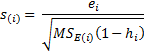
As we saw in Residuals, the standard error of the residual ei is
![]()
and so the studentized residuals si have the following property:
![]()
We will use this measure when we define Cook’s distance below. For our purposes now, we need to look at the version of the studentized residual when the ith observation is removed from the model, i.e.
where
![]()
i.e.
![]()
Cook’s distance and DFFITS
Definition 2: If we remove a point from the sample, then the equation for the regression line changes. Points that have the most influence produce the largest change in the equation of the regression line. A measure of this influence is called Cook’s distance. For the ith point in the sample, Cook’s distance is defined as
![]()
where ŷj(i) is the prediction of yj by the revised regression model when the point (x, …, xik, yi) is removed from the sample.
Another measure of influence is DFFITS, which is defined by the formula
![]() Whereas Cook’s distance is a measure of the change in the mean vector when the ith point is removed, DFFITS is a measure of the change in the ith mean when the ith point is removed.
Whereas Cook’s distance is a measure of the change in the mean vector when the ith point is removed, DFFITS is a measure of the change in the ith mean when the ith point is removed.
Observations about Cook’s distance
Property 1: Cook’s distance can be given by the following equation:
![]()
Property 1 means that we don’t need to perform repeated regressions to obtain Cook’s distance. Furthermore, Cook’s distance combines the effects of distance and leverage to obtain one metric. This definition of Cook’s distance is equivalent to
![]()
Values of Cook’s distance of 1 or greater are generally viewed as high.
Observations about DFFITS
Similarly, DFFITS can be calculated without repeated regressions as shown by Property 2.
Property 2: DFFITS can be given by the following equation:

Values of |DFFITS| > 1 are potential problems in small to medium samples and values of |DFFITS| > 2
Linear regression example
Example 1: Find any potential outliers or influencers for the data in Example 1 of Regression Analysis What happens if we change the Life Expectancy measure for the fourth data element from 53 to 83?
Figure 1 displays the various statistics described above for the data in Example 1.

Figure 1 – Test for potential outliers and influencers
Representative formulas in the worksheet in Figure 1 are displayed in Figure 2.
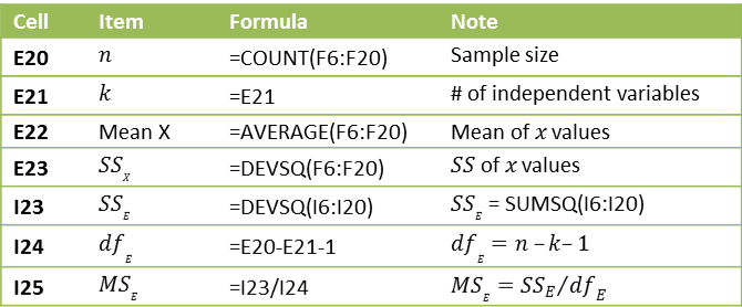
Figure 2 – Formulas in Figure 1
The formulas for the first observation in the table (row 6) of Figure 1 are displayed in Figure 3. The formulas for the other observations are similar.
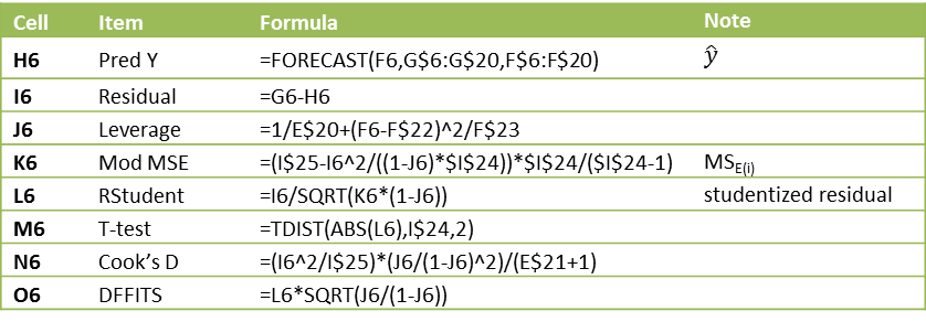
Figure 3 – Formulas for observation 1 in Figure 1
Analysis
As you can see, no data element in Figure 1 has a significant t-test (< .05) nor a high Cook’s distance (> 1) or DFFITS (> 1). We now repeat the same analysis where the Life Expectancy measure for the fourth data element (cell B9) is changed from 53 to 83 (Figure 4).

Figure 4 – Test for outliers and influencers for revised data
This time we see that the fourth observation has a significant t-test (.0096 < .05) indicating a potential outlier and a high Cook’s distance (1.58 > 1) and high DFFITS (2.71 > 1) indicating an influencer. Observation 13 also has a significant t-test (.034 < .05). Observations 3 and 14 are also close to having a significant t-test and observation 14 is close to having a high DFFITS value. The charts in Figure 5 graphically show the influence the change in observation 4 has on the regression line.

Figure 5 – Change in regression lines
We can also see the change in the plot of the studentized residuals vs. x data elements. Here it is even more apparent that the revised fourth observation is an outlier (in Version 2).

Figure 6 – Change in studentized residuals
In the simple regression case, it is relatively easy to spot potential outliers. This is not the case in the multivariate case. We consider this in the next example.
Multiple linear regression example
Example 2: Find any outliers or influencers for the data in Example 1 of Method of Least Squares for Multiple Regression.
The approach is similar to that used in Example 1. Figure 7 displays the output from the analysis.

Figure 7 – Test for outliers and influencers
The formulas in Figure 7 refer to cells described in Figure 3 of Method of Least Squares for Multiple Regression and Figure 1 of Residuals, which contain references to n, k, MSE, dfE, and Y-hat.
All the calculations are similar to those in Example 1, except that this time we need to use the hat matrix H to calculate leverage. E.g. to calculate the leverage for the first observation (cell X22) we use the following formula
=INDEX(Q4:AA14,Q22,Q22)
i.e. the diagonal values in the hat matrix contained in range Q4:AA14 (see Figure 1 of Residuals).
Alternatively, we can calculate the k × 1 vector of leverage entries, using the Real Statistics DIAG function (see Basic Concepts of Matrices), as follows:
=DIAG(Q4:AA14)
Note too that we have added the standardized residuals (column W), which we didn’t show in Figure 1. We use MSE as an estimate of the variance, and so e.g. cell W22 contains the formula =V22/SQRT($O$19), where cell O19 contains the MSE value (which is 34.6695).
Note that this estimate of variance is different from the one used in Excel’s Regression data analysis tool (see Figure 6 of Multiple Regression Analysis).
As we can see from Figure 7 there are no clear outliers or influencers, although the t-test for the first observation is .050942, which is close to being significant (as a potential outlier). This is consistent with what we can observe in Figure 8 of Multiple Regression Analysis and Figure 2 of Residuals.
Real Statistics Support
Real Statistics Function The Real Statistics Resource Pack provides the following array worksheet function where R1 is an n × k array containing X sample data.
LEVERAGE(R1) = n × 1 vector of leverage values
Real Statistics Data Analysis Tool: The Real Statistics Resource Pack also provides Cook’s D support which outputs a table similar to that shown in Figure 7.
To use this tool for Example 2, perform the following steps: Press the key sequence Ctrl-m and then select Multiple Linear Regression from the Reg tab (or from the Regression menu if using the original user interface). A dialog box will then appear as shown in Figure 2 of Real Statistics Capabilities for Multiple Regression. Next, enter A3:B14 for Input Range X and C3:C14 for Input range Y, click on Column Headings included with data, retain the value .05 for Alpha, select the Residuals and Cook’s D option, and click on the OK button. The output shown in Figure 8 is now displayed.
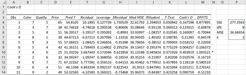
Figure 8 – Cook’s D output
These results are identical to those displayed in Figure 7 with the exception of column N of Figure 8. For any row in the output where either the p-value of the T-test < .05 or Cook’s D ≥ 1 or the absolute value of DFFITS ≥ 1 then an asterisk is appended to the output for that row. Since DFFITS = 1.09 ≥ 1, an asterisk appears in column N for the 7th observation (cell N10).
Real Statistics charts
In addition, when the Residuals and Cook’s D option is selected, two charts are output as shown in Figure 9. The chart on the right plots the fitted (i.e. predicted) y values versus the residuals and the chart on the left plots the fitted y values versus the studentized residuals (and so is identical to the chart in Figure 2 of Regression Residuals.
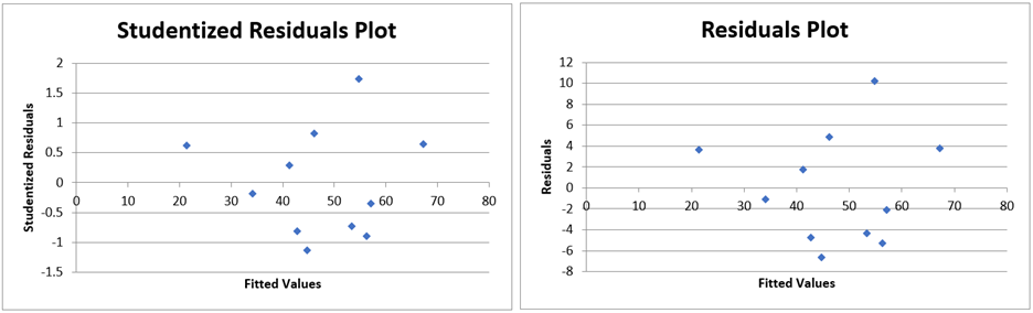
Figure 9 – Residuals
Examples Workbook
Click here to download the Excel workbook with the examples described on this webpage
References
Howell, D. C. (2010) Statistical methods for psychology (7th ed.). Wadsworth, Cengage Learning.
https://labs.la.utexas.edu/gilden/files/2016/05/Statistics-Text.pdf
Wikipedia (2012) Cook’s distance
https://en.wikipedia.org/wiki/Cook%27s_distance
Wikipedia (2012) DFFITS
https://en.wikipedia.org/wiki/DFFITS
Thanks for this great article. I’m trying to do weighted quadratic regression, i.e., instead of the input x_i and y_i, my actual inputs are w_i, w_i*x_i, w_i*x_i*x_i, w_i*y_i, where the weight w_i is the function of x_i, too. I set w_i=1/(abs(x_i)+0.1)^2) to focus the points around the origin point.
My question is, what is the right way to calculate the cooked distance in this case? Shall I just use x_i or y_i as if there is only one independent variable? Or I shall treat them as 3 variables?
Hello Jerron,
Can you please clarify the regression model? Do you have (1) two independent variables x and y (with the dependent variable z) or (2) one independent variable x (with dependent variable y)? Do you want the weights to apply to the independent variable(s) or both independent and dependent variables?
Charles
My study has 6X-Scores, how do I calculate the average? you used an X variable, how do I get more than one variable?
I am not familiar with 6X-Scores. Can you provide more information?
Charles
Dear Sir,
Can i use IQR method to detect outliers in regression analysis?
As we know, outliers are any observation that are below Q1 – 1.5IQR or above Q3 + 1.5IQR. Where, IQR = Q3 – Q1.
If this method is accepted for use, on which data set we detect for outliers? Only on x, or y, or both?
Thanks.
Dear Maaruf,
This approach can be used for any set. Note that the value 1.5 is somewhat arbitrary. 2.2 is often used instead.
Charles
This is a tremendous article; thank you for your guidance and for your great work as always, Dr. Zaiontz!
Hi Charles,
This is a follow up to my last question. The df for the internally studentized residuals are given as n-k-1 since it is t-distributed. So, should the df for the externally studentized residuals (deleted residuals) be n-k-2? Thanks for your help.
Tuba
Hello Tuba,
The df is as described on this webpage (esp. see the example).
Charles
Hi Charles,
I had a question for you regarding the distribution of the internally studentized residual vs the externally studentized residuals (deleted residuals). According to the references that I read, only the deleted residuals follow a t-distribution. The internally studentized residuals follow a more complex distribution (but almost t distributed) with critical values available from authors such as Lund (Lund, R. E., (1975). Tables for an approximate test for outliers in linear models. Technometrics, 17, 473-476). I guess the question is: how big is this difference or how significant is this difference in the critical values. What are your thoughts on this?
Tuba
Hi Tuba,
The t distribution can be calculated by Excel T.DIST function and the critical values by the T.INV function.
The Real Statistics website reviews the studentized distribution at the webpage
Studentized q Distribution
This webpage explains Real Statistics function QDIST and QINV that computes the studentized distribution values and critical values.
The table of critical values can be found at
Studentized Range Table
Charles
Charles,
Just bring up your attention on the summary data errors in Figure 4:
the values under the column Mod MSE should be corrected as follows:
97.68895647
96.82947122
79.45288209
67.90890458
90.70750869
94.59182394
94.02040728
95.52565913
96.6727156
97.77645285
90.80892708
97.81043162
75.9276476
81.04468244
89.36670749
As values in this column are not correct, the subsequent columns should be corrected accordingly.
-Sun
Hi Sun,
Yes, you are correct. For some reason the non-revised values were displayed. I have now corrected the webpage to display the revised values. Thanks for finding this mistake and thanks for your invaluable assistance in improving the website.
Charles
Charles,
Under Figure 7, you stated that “We use MSE as an estimate of the variance, and so e.g. cell W22 contains the formula =V22/SQRT($O$19). Note that this estimate of variance is different from the one used in Excel’s Regression data analysis tool (see Figure 6 of Multiple Regression Analysis).”
My questions for you are:
1. Why the MSE from the multiple linear regression has not been used for MSE in calculating the studentized residulas?
2. There is no cell $0$19 we can refer to in the current text calculating the denominator portion.
Thanks for your explanation in advance!
-Sun
Hi Sun,
1. It is the usual regression MSE except that it has been modified so that the data vector under consideration has been removed (similar to the way Cook’s distance is calculated).
2. Yes, this is confusing. The value of O19 is clear in the examples spreadsheet but not in the webpage. I have now corrected this. Thanks for pointing this out.
Charles
Hi again,
Sorry for the big numbers of questions (I do not have any question till I work with the data). Could you explain me a little the t test performed in this case? What is the nule hypothesis? Which data is used to perform this t test?
Thanks a lot
I have read this information:
“Since the deleted residuals follows the Student t distribution we can use a critical value based on Bonferroni correction”
This is the reference:
Cousineau, D., & Chartier, S. (2010). Outliers detection and treatment: a review. International Journal of Psychological Research, 3(1), 58-67.
Why those authors suggest to use Bonferroni correction?
Hello Gabriel,
This makes sense since there are multiple tests and so Bonferroni’s correction seems reasonable (provided the separate tests are independent). Having said this, I have not seen it applied in practice. Since these tests only identify potential outliers, without the Bonferroni correction more potential outliers would be identified. This doesn’t mean that the user needs to declare them as an outlier.
Charles
Thanks
Gabriel
Hi again Charles,
Another question,
I am performing regression with only one predictor… For deleting outliers what is better? Using the Cook’s distance, the DDFIT or the Pvalue that appear in the table when I use the Real Statistic App (here I pasted the mentioned table):
Obs X1 Y Pred Y Residual Leverage SResidual Mod MSE RStudent T-Test Cook’s D DFFITS
1 9.70622 109 92.07016707 16.92983293 0.167562181 2.243616618 40.03439335 2.932649393 0.008894744 0.608610861 1.315746566
2 9.8777 101 93.16957624 7.830423758 0.129453685 1.037722519 56.14496375 1.120041002 0.277419117 0.09197359 0.431911919
3 10.78357 85 98.97737765 -13.97737765 0.051628674 -1.852344137 48.17029702 -2.06798236 0.053323291 0.098479876 -0.482506431
4 10.62244 96 97.9443254 -1.944325398 0.050287629 -0.257670633 60.05395342 -0.257455456 0.799747393 0.001850874 -0.059242944
5 10.67227 100 98.26380032 1.736199684 0.050000586 0.23008889 60.10145528 0.229771156 0.820860422 0.001466526 0.052713444
6 11.64134 108 104.4767957 3.523204323 0.169355764 0.466910678 59.40905872 0.501538142 0.622071189 0.026755156 0.226462569
7 10.6005 102 97.80366155 4.196338453 0.050613257 0.556117401 59.19704414 0.559756205 0.58254519 0.008683223 0.129243729
8 11.17288 98 101.4733596 -3.473359592 0.081983919 -0.460305033 59.51506788 -0.469906158 0.644064898 0.010305986 -0.140426907
9 11.30398 100 102.3138806 -2.313880599 0.100838888 -0.306645729 59.93784093 -0.315189426 0.756242592 0.005864039 -0.105552107
10 10.9151 107 99.82065551 7.179344489 0.057594095 0.951438603 57.07087077 0.978945567 0.34058188 0.029351717 0.242007333
11 8.93155 74 87.1035278 -13.1035278 0.432462658 -1.736537676 42.49166606 -2.668327511 0.015669483 2.024408514 -2.32925062
12 10.19137 86 95.1806077 -9.1806077 0.0790014 -1.216654889 54.90497365 -1.291029307 0.213028866 0.068932124 -0.37811509
13 10.61712 98 97.9102173 0.089782701 0.050355399 0.011898402 60.28760557 0.011865829 0.990663188 3.95249E-06 0.002732377
14 10.4253 93 96.68040235 -3.680402353 0.057583869 -0.487743259 59.4426334 -0.491727983 0.628854414 0.007712017 -0.121549728
15 10.6616 102 98.19539178 3.80460822 0.05000918 0.504203571 59.39180869 0.506508761 0.618647456 0.007043569 0.116212307
16 10.58703 105 97.71730138 7.28269862 0.050873529 0.965135552 57.00101433 0.990122667 0.335238201 0.026302094 0.229230759
17 10.73626 102 98.6740592 3.325940803 0.050553563 0.44076844 59.60275927 0.442126044 0.663664303 0.005447557 0.102020336
18 11.44917 99 103.2447368 -4.244736777 0.126796137 -0.562531362 59.07433332 -0.591008226 0.561863608 0.026311052 -0.225210541
19 11.4189 102 103.0506668 -1.050666824 0.120944266 -0.139239032 60.21423547 -0.144413311 0.88677874 0.001517206 -0.053566301
20 11.08805 98 100.9294893 -2.929489287 0.07210132 -0.388228925 59.74406048 -0.393454274 0.698605431 0.00631085 -0.109677009
Hello Gabriel,
Cook’s distance and DFFITS are pretty similar measurements are used to identify leverage points. See, for example
https://en.wikipedia.org/wiki/DFFITS
The p-values are used to identify potential outliers.
Charles
Thanks very much Charles
Gabriel
Thanks Charles
Gabriel
Dear Charles,
I want to use this app to detect outliers in a regression but I have some blank cells… I do not want to delete the rows with the blank cells because it contains interesting values in other columns. I will explain with a simple example:
Weight / Heigh / Foot size
Imagine I want to find the correlation between the weight and the foot size and between the weight and the height… In subject number 1 I have the weight, and the height but not the foot size. In subject 4 I have the weight and the heigh but not the foot size. I do not want to delete any row (subject). How can I do this with your tool?
Correction:
Imagine I want to find the correlation between the weight and the foot size and between the weight and the height… In subject number 1 I have the weight, and the height but not the foot size. In subject 4 I have the weight and the foot size but not the height. I do not want to delete any row (subject). How can I do this with your tool?
Hello Gabriel,
If you just want to calculate the correlations, then you can simply use Excel’s CORREL function. It only uses pairs which are both numeric and non-blank. E.g. suppose that you have the following data in range A1:D5.
subj weight foot height
1 100 – 60
2 80 12 55
3 105 11 70
4 70 7 –
Then the correlation between weight and foot size is .576557 as calculated by =CORREL(B2:B5,C2:C5)
The correlation between weight and height is .866025 as calculated by =CORREL(B2:B5,D2:D5)
The correlation between foot size and height is -1 as calculated by =CORREL(C2:C5,D2:D5)
Charles
Thanks Charles,
I also want to compute the Cooks’ D to detect outliers…
I think the only way is to delete blank cells no?
Best regards,
Gabriel
Hello Gabriel,
In the current implementation of the Multiple Regression data analysis tool you would need to delete any row with a blank cell.
Charles
Fantastic instrument,
Thanks,
Gabriel
For a cautious use of Cook’s Distance, please see the section “Detecting highly influential observations” in “https://en.wikipedia.org/wiki/Cook%27s_distance”.
for Cook’s distance, please see the paper:
http://www.csam.or.kr/journal/view.html?doi=10.5351/CSAM.2017.24.3.317
Zang,
Thanks for sending this link to me and others in the community.
I appreciate your help in identifying articles that could be interesting to users of the website.
Charles
Dear Sir,
With the help of this article i could be able to calculate all the outliers & influencers in excel itself very systematically except DFbetas.
May I request you to please guide “how to calculate “DFbetas” values in excel as an another indicator of Outliers & influencers ?”
Waiting for your guidance.
Shivang,
DFBetas(i,j) = (b_j – b_j(i)) / (s(i) * sqrt(c_j)) where
i is the index to the ith row of data
j is the index to the jth regression coefficient b_j
b_j(i) = the jth regression coefficient where the regression is repeated with the ith row of data deleted
s(i) = the standard error for the regression with the ith row of data deleted
c(j) is the jth value on the diagonal of inverse of the matrix X’X where X is the design matrix for the data
I have not yet implemented this in Excel, but will eventually.
Charles
Leverage Value which is analysed by SPPS is different from this Leverage Values, what is the resason of this?
I don’t know since I don’t use SPSS. If you send me an Excel file with your data and calculations I will try to understand why there may be a difference.
Charles
I think it is because SPSS uses the
centered leverage = Leverage-1/n
Thanks Antonio for clarifying this. Is there an advantage of using the SPSS approach?
Charles
Hi
Your results in Figure 3 for Mod MSE, Rstudent , T-test and DFFITS are incorrect.
To calculate Mod MSE in Figure 3 you used MS = 63.5 from Figure 1 rather than MS=90.29 from Figure 3
Dear Charles, when reading about testing on residuals ,it is always stated about variance homegeneity in data, but it is not the case in surveying data. What would you sugest? Thank you.
Claudio,
Looking at residuals is important for many reasons, not just for analyzing homogeneity of variances.
I am not sure what you mean, by “What do you suggest?”, though.
Charles
Charles, I perfomed a least square adjustment where data have different variances applying a weight matrix(the inverse of covariance matrix) . Is it possible the qq plot of residuals when data have different variances? Do I have to standarize residuals first?
Claudio
Claudio,
Sorry, but I don’t understand your question. You are creating a QQ plot of what data?
Charles
sorry by the delay. data are a levelling network and I’m to use different methods tu find outliers. I’ll plot studentized residuals vs adjusted height differences .
thank you
Dear Sir,
With regards to Declan’s comment on the RStudent formula, I would be most grateful if you could let me know if it has been looked at.
Thanks for a brilliant site, makes it clear even to a maths dunderhead like me 🙂
Malcolm,
The only place I used RStudent is in the Residuals and Cook’s D data analysis tool, which I understood Declan thought was accurate. I also checked with Howell’s textbook to make sure that I implemented it correctly and found that it checked out perfectly.
Charles
Hi Charles,
Could you please provide me with some information on how I should delete outlier data in each data set other than multi regression?
Thanks,
Ehsan
Thanks for the reply Charles. Can you provide any insight into whether or not IVs are automatically excluded from the model if they have a high degree of multi-collinearity. It seems spss does this automatically and i’m thinking it could account for some difference. Also, is your’s a SS type III estimator?
Thanks again; Best, Phillip
Phillip,
Excel drops one the variables if there is perfect collinearity. Otherwise, Excel doesn’t do anything. See the webpage https://real-statistics.com/multiple-regression/collinearity/.
I am using SS type III, which is relevant for unbalanced ANOVA models. See https://real-statistics.com/multiple-regression/unbalanced-factorial-anova/.
Charles
Your equation for Mod MSE in Figure 3 has an error. You seem to have flipped df and MSe. Should be (I$25-I6^2/(1-J6)/I$24)*….
Kevin,
The formula I actually used (as shown in the Examples Workbook) is =(I$25-I6^2/((1-J6)*$I$24))*$I$24/($I$24-1). I believe this is the same as the formula you listed (let me know if this is not so). The formula that is shown in Figure 3 of the referenced webpage is wrong. I will correct this shortly. Thanks for catching this error.
Charles
Thanks for producing these Charles. Cool stuff! I’m running some Cook’s D compared to the Cook’s D output from SPSS. They are very close, but not exactly the same results. Any clues as to where the difference may be? (in my case, your Cook’s D results are slightly lower — from .001 to .01 lower — than the SPSS results; not a huge difference but it led to different classification of 1% of cases)
Phillip,
I don’t know what the difference is. I don’t have SPSS and so I can’t check. I will try to investigate this in the future.
Charles
Sir
You wrote: “cell W22 contains the formula =V22/SQRT($O$19)” Or should it be V22/SQRT($O$19*(1-hi))?
Colin
Colin,
Cell W22 only contains the standardized residual and so the formula is the one given. Perhaps I should have used STDRESID (or something similar) instead of SRESIDUAL to make it clear that the S stands for “standard” not “studentized”.
Charles