Basic Concepts
When creating a multiple regression model, we would sometimes like to determine how much each independent variable contributes to the model. One way to do this is to decompose R-square using the Shapley-Owen Decomposition.
If x1, x2, …, xk represent the independent variable and y is the dependent variable, then the partial R-square for variable xj can be calculated by
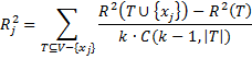
where V = {x1, x2, …, xk} and |T| = the number of elements in some subset T of V. Also R2(T) = the R-square value for the regression of the independent variables in T on y. We assume that R2(Ø) = 0.
To calculate the 
Example
Example 1: Find the Shapley-Owen decomposition for the linear regression for the data in range A3:D8 of Figure 1.

Figure 1 – Shapley-Owen Decomposition – part 1
We first calculate the R2 values of all subsets of {x1, x2, x3} on y, using the Real Statistics RSquare function. These values are shown in range G4:G11. We now apply the formula shown above for calculating
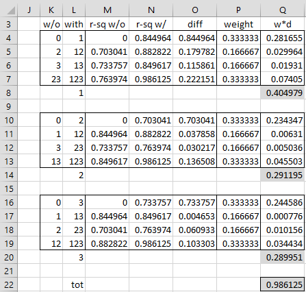
Figure 2 – Shapley-Owen Decomposition – part 2
Example Explanation
E.g. to calculate 
We see that 

Worksheet Function
Real Statistics Function: The Real Statistics Resource Pack contains the following array function. Here R1 is an n × k array containing the X sample data and R2 is an n × 1 array containing the Y sample data.
SHAPLEY(R1, R2): outputs an k × 1 column range containing the 
For Example 1, the output from the formula SHAPLEY(A4:C8,D4:D8) is shown in range G13:G15 of Figure 1.
Examples Workbook
Click here to download the Excel workbook with the examples described on this webpage.
Reference
Huettner, F. and Sunder, M. (2012) Stata module for decomposing goodness of fit according to Shapley and Owen values
https://www.stata.com/meeting/uk12/abstracts/materials/uk12_sunder.pdf
Great article, thanks so much!
Hi Charles,
Thank you for this. I manually replicated the results and completely grasped the concept of Shapley-Owen.
I wonder if there are similar metrics for Logistic Regression? I know the concept of pseudo R-Squared in Logistic Regression differs from the R-Square in Linear Regression, but are there any metrics to evaluate the importance of each IV and capture their specific impact in Logistic Regression models?
Hello Matthew,
I am not familiar with Shapley-Owen for logistic regression, but the following link provides some information and references.
https://rdrr.io/cran/sensitivity/man/lmg.html
Charles
Hi Charles,
Thanks for making this available. However, I am still having problems with the array. I Visited your page for Array Formula and Functions but I did not get it well.
How did you work the results for cell G8 with the formula “=RSquare(A4:B8, D4:D8). I keep getting an error.
Hi Eric,
The formula =RSquare(A4:B8, D4:D8) is not an array formula. You simply insert this formula in cell G8 and press Enter.
Charles
I have the same problem
Hi Nana,
Which version of Excel are you using?
Charles
Hi Charles, thank you for this. It has been invaluable in my understanding of Shapley-Owen.
Can you provide a bit of advice? Let’s say I have eight independent variables, which is more than I can do in Excel by hand. How can I make this process more manageable?
Hello Ralph,
I don-t know of an easier approach to use when you want to make the calculations by hand. I have provided the Real Statistics function so that you can easily make the necessary calculation.
Charles
Hello Charles,
I want first to thank you for providing us this kind of statistics.
As Henry already told you I don’t understand how to do without changing the data to have the results for the 2nd and the 3rd indicators.
I don’t understand how to use in this case Array Formulas and Functions.
Can you provide us an example (English is not my mother tong and it can be an explanation of my misunderstanding).
Regards
Sorry, but I don’t understand your comment.
Charles
Super useful, thanks for providing the examples and for creating the handy function. I noticed that the SHAPLEY function provides the Shapley result for the first column in the array (in your example A4:A8) but to get the results for the other columns (B4:B8 and C4:C8) I would need to rearrange the data array so that these columns come first. Is that correct or is there an easier way to indicate which column your referencing?
Also, is there a max array size that can be used? I am running on an array that is 22 columns by 50 rows of data and it is taking a significant time to return a result.
Hello Richard,
The SHAPLEY function is what Excel calls an array function, and so it will return the values for all the columns. You can’t simply press the Enter key, however, when using it. See the following webpage for how to use an array function:
Array Formulas and Functions
The max array size is much larger than 20 x 50. I don’t know how long it will take to generate the answer.
Charles
Sorry Charles, one more question – I’m a bit unclear about the weight column in your figure 2 excel example – I wasn’t clear how to translate k · C(k–1,|T|), into excel. From your numbers I noticed that the top/bottom rows were reproducible with 1/k and the middle rows 1/((k-1)*k). This worked for k=3 and k=4 but when I did k=5, the weights added to 1.1 so this does not seem to be the solution.
Are you able to explain the weight column a bit more?
Hello Henry,
First of all, for the case under consideration where k = 3, T can have either 0, 1 or 2 elements. For 0 elements, k · C(k–1,|T|) = 3 · C(2,0) = 3, and so the weight is 1/3. For 1 element, k · C(k–1,|T|) = 3 · C(2,1) = 6 and so the weight is 1/6. For 2 elements, k · C(k–1,|T|) = 3 · C(2,2) = 3 and so the weight is 1/3. There are C(2,0) = 1 case with 0 elements, C(2,1) = 2 cases with 1 element and C(2,2) = 1 case with 2 elements. Thus the sum of the weights is 1(1/3) + 2(1/6) + 1(1/3) = 1.
Now let’s look at the case where k = 5. T can have 0, 1, 2, 3 or 4 elements. The weights for each of these are the reciprocals of 5 · C(4,0) = 5, 5 · C(4,1) = 20, 5 · C(4,2) = 30, 5 · C(4,3) = 20, 5 · C(4,4) = 5, i.e. 1/5, 1/20, 1/30, 1/20 and 1/5. Assuming that variable 1 is under consideration, there is C(4,0) = 1 value of V with 0 elements, C(4,1) = 4 with 1 elements, C(4,2) =6 with 2 elements, C(4,3) = 4 with 3 elements and C(4,4) = 1 with 4 elements. Thus the sum of the weights = 1(1/5) + 4(1/20) + 6(1/30) + 4(1/20) + 1(1/5) = 1/5 + 1/5 + 1/5 + 1/5 + 1/5 = 1.
Charles
Thanks Charles,
I got that working using this formula for the weight:
1/(k*(fact(k-1)/(fact(n)*fact(k-1-n))))
where k is the number of variables and n is the number of items in the w/o column.
Hi Charles,
Thanks very much for making this available.
I have been putting together a workbook to handle many independent variables and decided it was best to avoid copying the non-contiguous variable combinations due to the number of permutations. I thought it would be possible to use named ranges but I find they give different results.
eg with your test data above – x1 against x3 R-sq = 0.849617
but if I create a named range of the x1 and x3 data and use that in the formula I get 0.844964
Do you know why the named range doesn’t work the same in the formula – is there no way to use that approach?
Henry,
The problem is not with using a named range. The problem is that the Real Statistics formula only recognizes a contiguous range. You can use the SelectCols array function to create a contiguous array and then use other Real Statistics functions on the result.
Charles
Thanks very much for your quick assistance Charles, I’ll have a look into function.
Hi Charles,
When I use the SHAPLEY function I recive as output only one number in one cell but not ther full range (in your example, only G13, but not G14 and G15).
There is something that I do wrong?
Thanks
Ruben,
This is because SHAPLEY is an array function. To see how to get all the output, see the following webpage:
Array Formulas and Functions
Charles