LAD Regression is based on minimizing the absolute value of the residuals; i.e. the least absolute deviation, which uses the Lp norm where p = 1, as described in Lp Norm. Ordinary least squares regression is based on minimizing the mean squared error (MSE) statistic, which is based on the Lp norm where p = 2.
On this webpage, we describe Lp regression, which is similar to LAD regression, and uses IRLS and bootstrapping, and is based on the Lp norm but where p can take any value between 1 and 2 (instead of L1 = MAE).
Data Analysis Tool
Real Statistics Data Analysis Tool: The LAD Regression data analysis tool, described in LAD Regression Analysis Tool, also supports Lp regression. The p field, as described in Figure 1 of LAD Regression Analysis Tool, is simply set to the desired value of p instead of the default value of 1 as for LAD regression.
For example, when p is set to 1.5, instead of 1, for Example 1 of LAD Regression Using IRLS, we obtain the output shown in Figure 1.
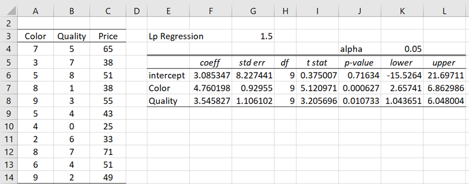
Figure 1 – Lp regression
Worksheet Functions
Real Statistics Functions: For the following array functions, R1 is an n × k array containing the X sample data, R2 is an n × 1 array containing the Y sample data, con = TRUE (default) if a constant term is included, p specifies the Lp norm to be used, and iter is the number of iterations performed (default 25).
LpRegCoeff(R1, R2, con, p, iter) = column array consisting of the regression coefficients; if con = TRUE, then the output is a k+1 × 1 array, while if con = FALSE, it is a k × 1 array
LpRegWeights(R1, R2, con, p, iter) = n × 1 column range consisting of the weights calculated from the iteratively reweighted least-squares algorithm
LpRegCoeffSE(R1, R2, con, p, iter, nboots) = column array consisting of the standard errors of the regression coefficients; if con = TRUE, then the output is a k+1 × 1 array, while if con = FALSE, it is a k × 1 array; nboots = the number of bootstraps (default 500)
Further explanation is provided at LAD Regression Using IRLS and LAD Regression Standard Errors for the case where p = 1 and Lp regression is equivalent to LAD regression.
Examples
In Figure 2, range I6:I8 specifies the Lp regression coefficients when p is set to 1.5. It contains the array formula =LpRegCoeff(A4:B14,C4:C14,,I4,25).
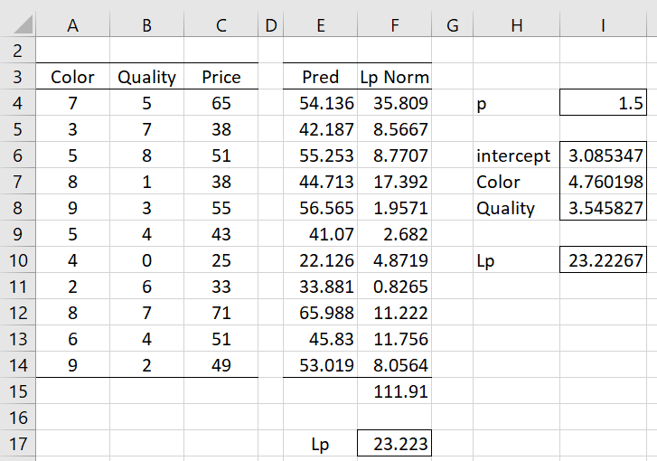
Figure 2 – LpRegCoeff
The prices predicted by the Lp regression model are shown in column E of Figure 2; e.g. cell E4 contains the formula =$I$6+A4*$I$7+B4*$I$8. The absolute values of the residuals raised to the pth power are shown in column F; e.g. cell F4 contains the formula =ABS(C4-E4)^$I$4. The sum of these values is shown in cell F15, as calculated via the formula =SUM(F4:F14). Finally, the Lp norm value (similar to the MSE value when p = 2 and MAE value when p = 1) of 23.2267 is shown in cell F17, which contains the formula =F15^(1/I4).
This value can also be calculated via the formula
=SUMPRODUCT(ABS(C4:C14-MMULT(DESIGN(A4:B14),I6:I8))^I4)^(1/I4)
as shown in cell I10.
Examples Workbook
Click here to download the Excel workbook with the examples described on this webpage.
References
Wikipedia (2016) Least absolute deviations
https://en.wikipedia.org/wiki/Least_absolute_deviations
Wikipedia (2016) Iteratively reweighted least squares
https://en.wikipedia.org/wiki/Iteratively_reweighted_least_squares
Thanoon, F. H. (2015) Robust regression by least absolute deviations method
http://article.sapub.org/10.5923.j.statistics.20150503.02.html