Basic Concepts
We now explore another measure of central tendency that is robust to outliers. This measure is based on the Lp norm, which for a vector X = (x1, …, xn) is defined by
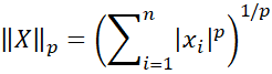
The Minkowski distance between vectors X and Y is defined as ||X–Y||p. When p = 2, this is the usual Euclidean distance, and when p = 1, this is often referred to as the Manhattan distance (aka the city block distance or taxicab distance).
If y is a scalar, then ||X–y||p = ||X–Y||p, where Y is the vector all of whose elements are y.
Note that
![]()
Actually, when p = 1, if X has an even number of elements, then any y between the two middle values would minimize the norm (not just the average of these values, as for the median).
The mean gives too much weight to outliers, while the median gives no weight to outliers. We, therefore, propose using the following statistic as a robust measure of central tendency for values of p between 1 and 2. Here, we are looking for a Goldilocks value that doesn’t give too much weight to outliers but also doesn’t discount outliers completely.
Values of p closer to 1 give less weight to outliers, while values of p closer to 2 give more weight. Note that if X = (1, 2, 9), the median gives no weight to the 9, while L1.2(X) = 2.023 gives some weight to the 9, but not too much. If X = (1, 2, 12), then L1.2(X) = 2.061 gives a little more weight to the 12 than to the 9, but again not too much.
Example
Example 1: Calculate L1.2(X) for X = (1, 2, 12) using Solver.
Set up Excel’s Solver as described in Figure 1. We start with an initial guess for x = L1.2(X) in cell E5 of 5 (mean of the values in X). Our goal is to minimize the value in cell E6 by changing the value in cell E5. Note that cell B4 contains the worksheet formula =ABS(A4-$E$5)^$E$4.
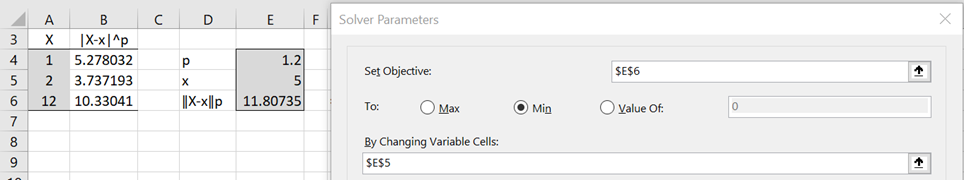
Figure 1 – Initialization of Solver
The result from Solver is shown in Figure 2, namely, L1.2(X) = 2.060751, as shown in cell E5.
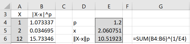
Figure 2 – Solver results
Observations
We can obtain the same results using Newton’s method as explained in Lp estimation via Newton’s Method.
In the case where X has an even number of elements and the median is halfway between a and b, with b the next largest element in X after a, then L1(X) can take any value between a and b and not just (a+b)/2.
Worksheet Functions
Real Statistics Functions: The following functions are provided in the Real Statistics Resource Pack.
LpEST(R1, p, R2, iter, guess, check) = Lp(X) where X = the data in the column array R1.
Here, 1 ≤ p ≤ 2, iter = the number of iterations (default 100) used to find the value of y that minimizes ||X–y||p, and guess is an optional initial guess of this value. If check = TRUE (default FALSE), then this function returns a 2 × 1 array whose second value should be near zero as a check that the iteration has converged.
R2 is an optional column array containing weights. R2 contains the same number of elements as R1. See Weighted Minkowski Distance for a description of the weighted version of Lp(X).
LpNORM(R1, R2, p, R3) = the Minkowski distance between the column arrays R1 and R2; R1 and R2 have the same number of elements.
If R2 is a scalar then R2 is treated as a column array all of whose values are this scalar. R3 is an optional column array containing weights. R3 contains the same number of elements as R1. See Weighted Minkowski Distance for a description of the weighted Minkowski distance.
Using worksheet formulas
For Example 1, the formula =LpEST(A4:A6,1.2) returns the value shown in cell E5 of Figure 2. The Minkowski distance between the vector A4:A6 and the value of L1.2(X) shown in cell E5 can be calculated by the formula =LpNORM(A4:A6,E5,1.2), returning the value shown in cell E6 of Figure 2.
The Euclidean distance between the points (2, 3) and (4, 5) is the square root of (4-2)2+(5-3)2 = 2.828. The same value is obtained using the formula =LpNORM(R4:R5,S4:S5,2) as shown in Figure 3.
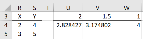
Figure 3 – Minkowski distance
The taxicab distance is 4 (equivalent to 4 city blocks, 2 horizontally plus 2 vertically) using the formula =LpNORM(R4:R5,S4:S5,1). When p = 1.5, the Minkowski distance is 3.175 using the worksheet formula =LpNORM(R4:R5,S4:S5,1.5).
Measure of Variability
Since the population variance of X is the mean of the values (xi – x̄)2, we can calculate the population variance by the array formula =LpEST(ABS(R1-LpEST(R1,2))^2, 2). Similarly, we can calculate the MAD statistic by =LpEST(ABS(R1-LpEST(R1,1))^1, 1). Thus, we can use the following formula as a measure of variability for any p: =LpEST(ABS(R1-LpEST(R1,p))^p, p).
Chebychev Norm and Distance
The Chebychev norm is the Lp norm where p = ∞. Actually ||X||∞ is defined as the limit of ||X||p as p → ∞. This is equivalent to the maximum of the |xi| for i = 1, …, n. The Chebychev distance is defined similarly.
Starting with Rel 9.9, the LpNORM worksheet function will support the Chebychev and weighted Chebychev distance. In this case, the p argument is set to zero (instead of infinity).
Links
Examples Workbook
Click here to download the Excel workbook with the examples described on this webpage.
References
Zornoza, J. (2020) Distance metric for machine learning. Aigents
https://aigents.co/data-science-blog/publication/distance-metrics-for-machine-learning
Wikipedia (2020) Minkowski distance
https://en.wikipedia.org/wiki/Minkowski_distance