The Excel model described in Exponential Regression using a Linear Model suffers from the shortcoming that it doesn’t actually minimize the sum of the squares of the deviations. We now show how to use Solver to create a better, nonlinear, regression model.
Example
Example 1: From the data for Example 1 of Exponential Regression using a Linear Model, as shown in range A3:B14 of Figure 1, we construct the other entries in Figure 1 (see also Figure 2). Our goal is to minimize the value in E15.
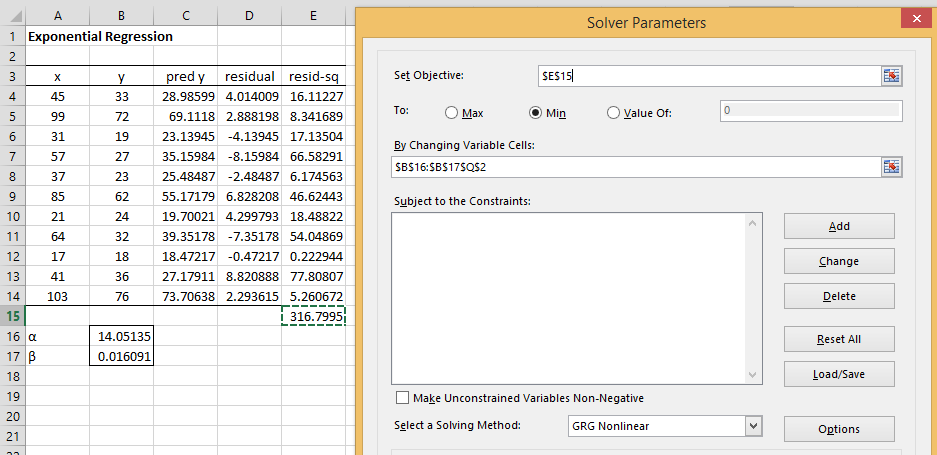
Figure 1 – Exponential Regression via Solver
Key formulas from Figure 1 are shown in Figure 2.
| Cells | Item | Formula |
| C4 | ŷ1 | =$B$16*EXP($B$17*A4) |
| D4 | y1 − ŷ1 | =B4-C4 |
| E4 | (y1 − ŷ1)2 | =D4^2 |
| E15 |  (yi − ŷi)2 (yi − ŷi)2 |
=SUM(E4:E14) |
Figure 2 – Key formulas from Figure 1
The initial values of the regression coefficients are taken from the coefficients calculated by Excel as shown in Figure 2 or 4 of Exponential Regression using a Linear Model, namely α = EXP(2.6427) = 14.05135 and β = .016091.
Solver Results
We now employ Excel’s Solver by selecting Data > Analysis|Solver. Next fill in the dialog box that appears as shown on the right side of Figure 1 and press the OK button. The result is shown in Figure 3. Note that the deviation value in cell E15 has been reduced from 316.7995 (the value calculated using the Excel exponential regression procedure) to 299.165.
Also, note that the revised values of the regression coefficients are α = 13.50475 and β = .016854.

Figure 3 – Exponential Regression output
Examples Workbook
Click here to download the Excel workbook with the examples described on this webpage.
Link
Reference
Howell, D. C. (2010) Statistical methods for psychology (7th ed.). Wadsworth, Cengage Learning.
https://labs.la.utexas.edu/gilden/files/2016/05/Statistics-Text.pdf
Kaw, A., Nguyen, D. (2026) Nonlinear regression
https://math.libretexts.org/Workbench/Numerical_Methods_with_Applications_(Kaw)/6%3A_Regression/6.04%3A_Nonlinear_Regression
My first question is answered widely here.
By the way I had an error in my email that I correct now.