Goodness of Fit Tests based on the Characteristic Function

Basic Approach

The characteristic function of a probability distribution uniquely determines the characteristics of the probability distribution. We won’t get into the details about the characteristic function, but we will use a goodness-of-fit test based on the characteristic function.

To test whether a data set X = {x₁, …, x_n} fits a particular distribution ψ(θ₁, θ₂), we use the following steps:

1. Estimate the distribution parameters θ₁ and θ₂ based on the data in X (e.g. using the method of moments or MLE). Here θ₁ is a location parameter for the specified distribution and θ₂ is a scale parameter for the distribution.
2. Normalize the data by replacing each data element x_i by z_i = (x_i–θ₁)/θ₂
3. Calculate the test statistic I based on the values in X and the specific distribution. The form of I varies from distribution to distribution and is based on the characteristic function of the distribution.
4. Calculate the critical value I_α for α = .05 and .10 based on the specific distribution and the number of elements n in X.
5. If I ≥ I_α then reject the null hypothesis that the data in X fits the distribution.

The value of I_α is calculated via a function of the form

On this webpage, we describe how to perform this test for n between 10 and 400 for the normal and lognormal distributions.

On subsequent webpages, we describe how to perform this test for the following continuous distributions, using the normal test as a template: lognormal, uniform, exponential, Laplace, Logistic, Weibull, Cauchy, and multivariate normal.

Normal Distribution

To test whether data X = {x₁, …, x_n} fits a normal distribution with pdf

we use the estimates

and the test statistic

The values of I_α are calculated via

which we will represent by the following table

If I ≥  I_α, then we reject the null hypothesis that the data comes from a normal distribution.

Example

Example 1:  Repeat Example 1 of Shapiro Wilk Original Test using the Characteristic Function GoF test (the data is repeated in range B3:B14 of Figure 1).

The other elements in Figure 1 are obtained as follows. Insert =(B3-C$16)/C$17 in cell C3, highlight C3:C14 and press Ctrl-D. Next, insert the array formula =TRANSPOSE(C3:C14) in D2:O2. Then place the formula =EXP(-((C3^2)/6)) in cell P3, highlight P3:P14, and press Ctrl-D. Finally, insert the formula =IF(D$1<$A3,EXP(-(($C3-D$2)^2)/4),””) in cell D3, highlight D3:O14, and press Ctrl-R and Ctrl-D.

Figure 1 – GoF (part 1)

The analysis continues in Figure 2.

Figure 2 – GoF (part 2)

We see from Figure 2 that I = .029256 < .091759 = I_.10, and so we can’t reject the null hypothesis that the data is normally distributed.

Worksheet Function

Real Statistics Function: The Real Statistics Resource Pack provides the following worksheet array function to carry out the goodness of fit test.

ICF_GOF(R1, dist, lab, iter, param1, param2): returns a column array with the values I-stat, I-crit for alpha = .05 and .10 for the distribution specified by dist and the data in the column array R1 (with 10 to 400 elements).

The arguments for this function are similar to those for ADTEST (see One Sample Anderson-Darling Test). In particular, dist takes the values shown in Figure 3.

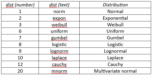
Figure 3 – dist values

Other Function Arguments

If the param1 and param2 arguments are set, then these values are used as the θ₁ and θ₂ parameter values respectively. If they are not set then iter is used to estimate these values as described next.

iter is used to determine the distribution parameters for the specified distribution (defined by dist). If iter > 0 then these parameters are estimated using the maximum likelihood estimate (MLE) based on the WEIBULL_FIT, etc. functions using the default argument values except that the number of iterations is set to the iter value (see Distribution Fitting via the MLE).

If iter = 0 or -1 then the distribution parameters are estimated using the method of moments based on the WEIBULL_FITM, etc. functions using the default argument values except that if iter = -1 then the pure argument is set to TRUE (see Distribution Fitting via the Method of Moments).

For the Cauchy distribution (dist = 12 or “cauchy”), then if iter = 0, then the trim mean estimate is used, while if iter = -1 then the median estimate is used; in either case, the exclusive version of the IQR is used.

If iter = -2 then the distribution parameters are estimated by the WEIBULL_FITR and CAUCHY_FITX functions using the default arguments. In fact, iter = -2 is only used for the Weibull and Cauchy distributions.

The formula =ICF_GOF(B3:B14,”norm”,TRUE,0) will produce the results shown in range R11:S13 of Figure 2.

Example

Example 2: Determine whether the data in column B of Figure 4 is normally distributed.

This time we use the ICF_GOF function to determine whether the data is normally distributed. Since I = .504308 > .32454 = I_.05, we reject the null hypothesis that the data comes from a normally distributed population. This is consistent with the results from the Shapiro-Wilk and d’Agostino-Pearson tests.

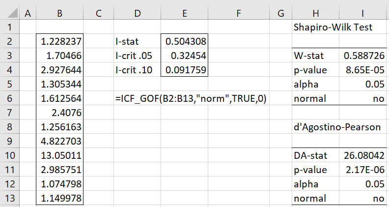
Figure 4 – ICF_GOF Function

Actually, the data in column B come from a Pareto distribution with m = 1 and α = 2.

Lognormal Distribution

Data X = {x₁, …, x_n} follows a lognormal distribution provided {ln x₁, …, ln x_n} follows a normal distribution.

Example 3: Determine whether the data in column B of Figure 5 comes from a lognormal distribution.

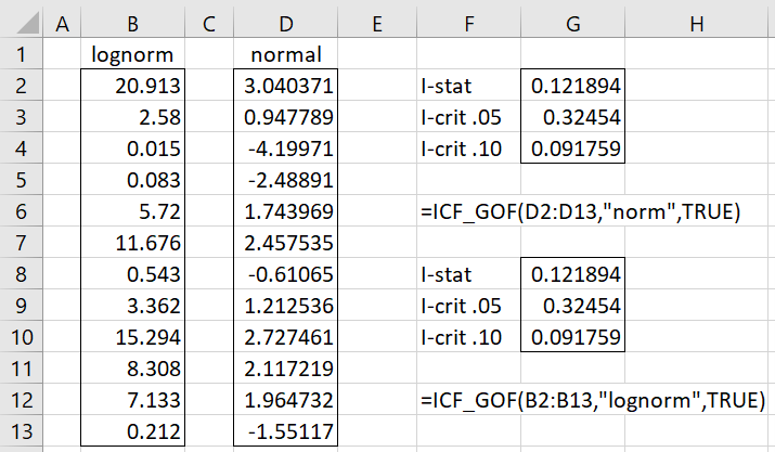
Figure 5 – GoF for the lognormal distribution

We use a log transformation as shown in column D of Figure 5 (e.g. cell D2 contains the formula =LN(B2)), and then test whether the transformed data is normally distributed. 

We see from Figure 5 that I = .121894 > .091759 = I_.10, and so we have a significant result at the .10 level. But also I = .121894 < .32454 = I_.05, which is not significant at the .05 level.

We get the same result by using the formula =ICF_GOF(B2:B13,”lognorm”,TRUE).

Examples Workbook

Click here to download the Excel workbook with the examples described on this webpage.

Reference

Epps, T. W. (2014) Probability and statistical theory for applied researchers
https://books.google.co.uk/books?id=NCs8DQAAQBAJ&pg=PR4&lpg=PR4&dq=Epps,+T.+W.+Probability+and+statistical+theory+for+applied+researchers&source=bl&ots=GxU40vCNHu&sig=ACfU3U0vgZZndBfjMMmqYPQuCXAJf2jrow&hl=en&sa=X&ved=2ahUKEwiw5_3R-4KCAxVCgFwKHa2fA384FBDoAXoECAQQAw#v=onepage&q=Epps%2C%20T.%20W.%20Probability%20and%20statistical%20theory%20for%20applied%20researchers&f=false