Introduction
Elsewhere on the website, we describe two methods for fitting data to a Cauchy distribution: the method of moments and maximum likelihood estimation (MLE). We now describe another approach based on order statistics.
Weighted Order Statistics Estimate
As usual, our objective is to identify the Cauchy distribution parameters μ and σ that result in a good fit for the data. Let’s assume that the data x1, …, xn is ordered so that x1 ≤ ⋅⋅⋅ ≤ xn.
For each i = 1, …, n, define
![]()
Next, define the following weights
![]()
The estimates for the parameters are
![]()
Worksheet Function
Real Statistics Function: The Real Statistics Resource Pack provides the following array function.
CAUCHY_FITX(R1, lab): returns a column array with the ordered statistics estimates of the mu and sigma parameters of the Cauchy distribution that best fits the data in the column array or range R1, along with the log-likelihood estimate based on these parameters. If lab = TRUE (default FALSE) then a column of labels is appended to the output.
Example
Example 1: Determine the parameters of a Cauchy distribution that best fit the data in range D2:H5 of Figure 1 using the various distribution fitting approaches described above.
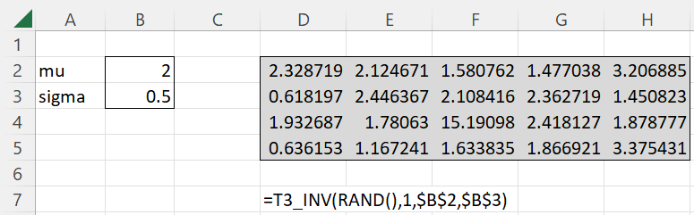
Figure 1 – Fitting data to a Cauchy distribution
We first note that the data in D2:H5 was obtained from a Cauchy distribution with mu = 2 and sigma = .5 by using the formula =T3_INV(RAND(),1,B2,B3) in all the cells of D2:H5. Thus, we expect that we will get a good fit for the data with a Cauchy distribution.
Figure 2 shows the results of fitting the data to a Cauchy distribution using the MLE, pseudo-method-of-moments, and ordered statistics approaches.
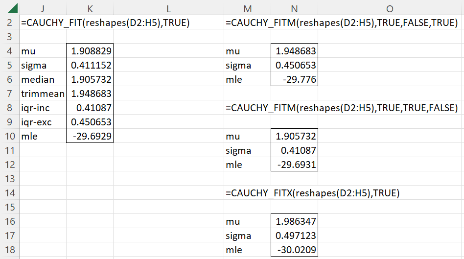
Figure 2 – Estimating Cauchy distribution parameters
The results are fairly similar, although we see that the ordered statistics approach yields estimates for the parameters that are closest to those in cells B2 and B3. Not surprisingly, though, the MLE approach yields the results with the largest log-likelihood value.
Examples Workbook
Click here to download the Excel workbook with the examples described on this webpage.
References
D’Agostino, R. B., Stephens, M. A. (1986) Goodness-of-fit techniques. Marcel Dekker, Inc.
https://www.hep.uniovi.es/sscruz/Goodness-of-Fit-Techniques.pdf
Chemoff, H., Gastwirth, J. L., Johns, M. V. (1967) Asymptotic distribution of linear combinations of functions of order statistics with applications to estimation. Ann. Math. Statist. 38, 52-73.
https://projecteuclid.org/journals/annals-of-mathematical-statistics/volume-38/issue-1/Asymptotic-Distribution-of-Linear-Combinations-of-Functions-of-Order-Statistics/10.1214/aoms/1177699058.full