We now extend the goodness-of-fit test based on the characteristic function to uniform and exponential distributions.
Uniform Distribution
For data X = {x1, …, xn} from a (continuous) uniform distribution on (a, b) with pdf
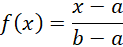
we use the estimates
a = min X b = max X
Now define

Thus

Define
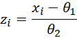
We use the test statistic
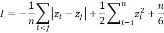
The critical values Iα of this statistic for 10 ≤ n ≤ 400 are


Henceforth, we will abbreviate these critical values as

If I ≥ Iα, then we reject the null hypothesis that the data come from a uniform distribution.
Example 1: Determine whether the data in column B of Figure 1 are uniformly distributed.
The analysis is also shown in Figure 1. Note that cell C3 contains the formula =(B3-C16)/C17 and cell D3 contains the formula =IF(D$1<$A3,ABS($C3-D$2),””). The other formulas in C3:M12 are filled in as explained in Example 1 of Goodness-of-Fit Test based on the Characteristic Function.
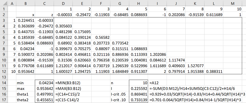
Figure 1 – GoF for uniform distribution
We see from Figure 5 that I = .225592 < .733139 = I.10, and so we can’t reject the null hypothesis that the data is uniformly distributed.
We get the same results as shown in range G14:H17 via the array formula =ICF_GOF(B3:B12,”uniform”,TRUE). See Goodness-of-Fit Test based on the Characteristic Function for a description of the ICF_GOF function and its arguments.
Note that if we test the 10 data elements in B2:B11 of Figure 1 via the formula =ICF_GOF(B2:B11,”uniform”,TRUE), we obtain I-stat = 2.963459 > .869401 = I.05. This is a significant result, providing evidence that the data are not uniformly distributed.
Exponential Distribution
For data X = {x1, …, xn} from an exponential distribution with pdf

We use the following MLE parameter estimates

The test statistic for this test is

The critical values when μ is unknown are

When μ is known, then use the above table assuming n = 0 (i.e. I.05 = .785 and I.10 = .635).
Example
Example 2: Decide whether the data in B3:B12 of Figure 2 fits an exponential distribution.
This example comes from the referenced textbook. Figure 2 describes the analysis. Note that cell C3 contains the formula =(B3-C16)/C17 and cell D3 contains the formula =IF(D$1<$A3,EXP(-ABS($C3-D$2)),””). The other formulas in C3:M12 are filled in as explained in Example 1.
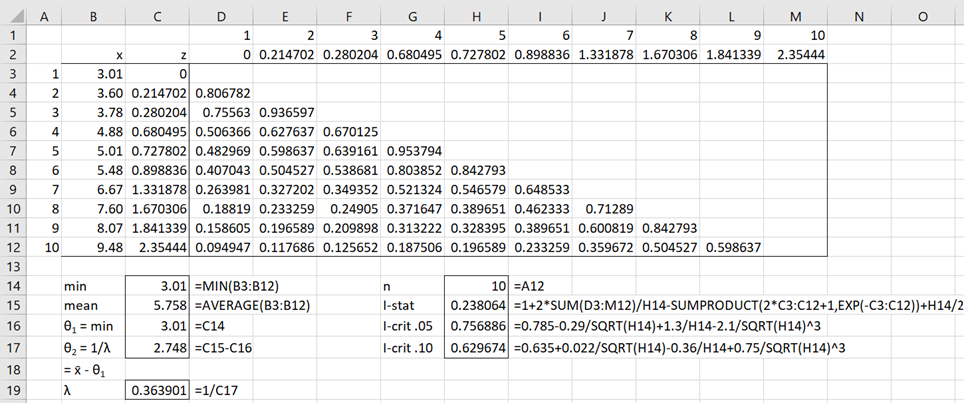
Figure 2 – GoF for Exponential distribution
We see from Figure 2 that I = .238064 < .629674 = I.10, and so we can’t reject the null hypothesis that the data is uniformly distributed with pdf
f(x) = .363901e–.363901(x–3.01)
We get the same results as shown in range G14:H17 via the array formula =ICF_GOF(B3:B12,”expon”,TRUE).
If instead, we know that μ = θ1 = 0, then using the worksheet formula =ICF_GOF(B3:B12,”expon”,TRUE,,0) we see that I = 1.189405 > 785 = I.05, and so p-value < .05, which is a significant result. Here we estimate λ = 1/5.758 = .173671. Thus, we conclude that the data doesn’t follow an exponential distribution, estimated by
f(x) = .173671e–.173671x
Links
↑ GoF tests using characteristic function
Examples Workbook
Click here to download the Excel workbook with the examples described on this webpage.
Reference
Epps, T. W. (2014) Probability and statistical theory for applied researchers
https://books.google.co.uk/books?id=NCs8DQAAQBAJ&pg=PR4&lpg=PR4&dq=Epps,+T.+W.+Probability+and+statistical+theory+for+applied+researchers&source=bl&ots=GxU40vCNHu&sig=ACfU3U0vgZZndBfjMMmqYPQuCXAJf2jrow&hl=en&sa=X&ved=2ahUKEwiw5_3R-4KCAxVCgFwKHa2fA384FBDoAXoECAQQAw#v=onepage&q=Epps%2C%20T.%20W.%20Probability%20and%20statistical%20theory%20for%20applied%20researchers&f=false