Overview
Assume that we have a random sample S = {x1, …, xn} and that^θ is the estimate of some parameter θ based on this sample using some function f(S).
The bootstrap estimate θ* of this parameter is obtained by creating a large number of bootstrap samples S1, …, Sm, where each Sj consists of n elements selected randomly from S with replacement. This results in m values θ1*, …, θm* where each θj* = f(Sj).
The bootstrap estimate θ* of θ is simply the mean of the θj*
![]()
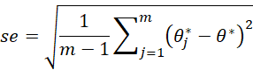
We can also obtain an estimate of the standard error of θ by using the standard deviation of the θj*
Percentile Confidence Interval
We can use (Clower, Cupper) an estimate of the 1 – α confidence interval of θ where
![]()
![]()
![]()
We will call this the percentile estimate of the confidence interval.
BCa Confidence Interval
Another estimate of the confidence interval, called the bootstrap bias-corrected and accelerated (BCa) confidence interval, can often produce less biased results. To obtain this confidence interval, we first need to define the median bias z0, and the acceleration a. The median bias is defined from the bootstrap using the inverse of the standard normal distribution, namely
![]()
and
![]()
The acceleration is defined using the jackknife sample of sample S (see Jackknife), as follows
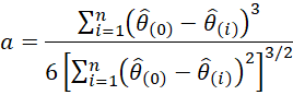
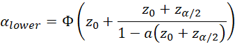
We now define the BCa confidence interval as the percentile confidence interval (Cα-lower, Cα-upper) where
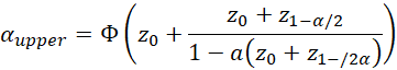
and
![]()
Worksheet Functions
Real Statistics Functions: The Real Statistics Resource Pack provides the following lambda array functions.
BOOTSTRAP(R1, expression, iter, ref): returns a column array with a bootstrap sample for the data in R1 based on the function f(arr) on a variable arr that takes array values; expression is used to specify f and ref is an optional reference to arr.
R1, expression, and ref are as for JACKKNIFE. iter is the number of bootstrap samples returned (default 2,000).
If R1 is a column array with elements S = {x1, …, xn}, then bootstrapping works by creating iter data sets S1, …, Siter where each Sj is formed by taking n elements from S with replacement. The bootstrap sample is then a column array containing the elements f(S1), …, f(Siter).
If R1 is an array with multiple columns, then the same approach is used except that now the xi represent rows in R1.
See Real Statistics Lambda Capabilities for additional information about lambda functions.
Confidence Intervals
The Real Statistics Resource Pack also provides the following lambda worksheet function.
CI_BOOTSTRAP(R1, expression, lab, iter, alpha, ref): returns various statistics resulting from a bootstrap sample for the data in R1 based on the function f(arr) on a variable arr that takes array values; expression is used to specify f, and ref is an optional reference to arr.
R1, expression, ref, and iter are as for BOOTSTRAP. alpha takes a value between 0 and .5 (default .05).
This function returns the following statistics:
- parameter estimate = f(arr) where arr is the R1 array
- bootstrap estimate = the average of the f(S1), …, f(Siter) for bootstraps Sj
- standard error = the standard deviation of the f(S1), …, f(Siter)
- percentile confidence interval (% lower, % upper) where % lower = the alpha*iter smallest value of f(Sj) and % upper = the alpha*iter largest value of f(Sj)
- BCa (bias-corrected and accelerated) confidence interval (BCa lower, BCa upper) = the BCa adjusted value of the percentile confidence interval
If lab = FALSE (default), then the output consists of a column array with the above 7 entries. If lab = TRUE, then an extra column is appended to the output consisting of labels.
Example
Example 1: Use bootstrapping to estimate the 95% confidence interval for the population mean, based on the data in range B1:M1 of Figure 1. Note this is the same data as shown in column B in Figure 1 of Jackknife.
We begin by creating a bootstrap with 2,000 bootstrap samples, as shown in the rows of range B2:M2001 of Figure 1 (only the first 15 samples are displayed). This is done by placing the array formula =RANDOMIZES(B1:M1) in array B2:M2, highlighting range B2:M2001, and pressing Ctrl-D. We then place the formula =AVERAGE(B1:M1) in cell N1, highlight the range N1:N2001, and press Ctrl-D.
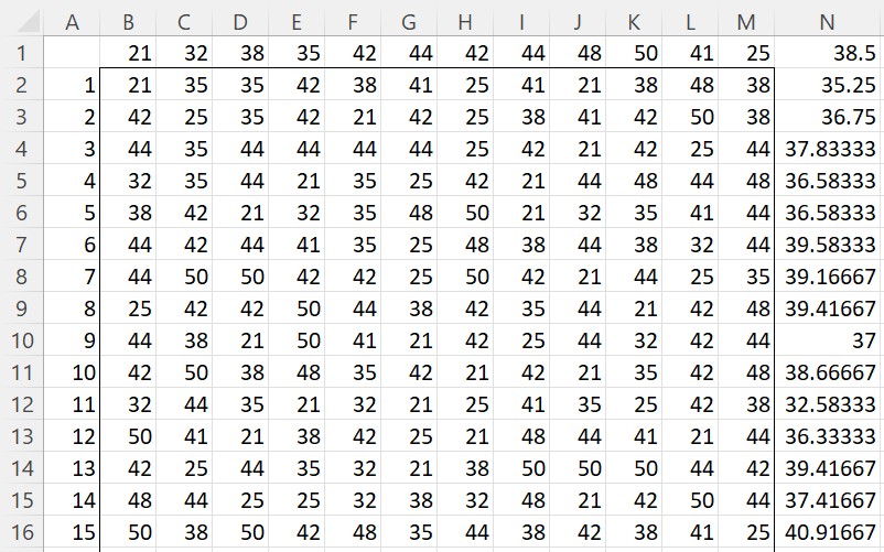
Figure 1 – Bootstrap sample
Here, N1 contains the mean of the original sample, and N2:N2001 contains the means from the 2,000 bootstrap samples. Alternatively, we can obtain the bootstrap sample shown in N2:N2001 by using the lambda formula
=BOOTSTRAP(TRANSPOSE(B1:M1),”=AVERAGE($arr)”)
Confidence Intervals
We now obtain the 95% confidence intervals based on the bootstrap, as displayed in Figure 2. The percentile confidence interval of (33.41667, 43.16667) is shown in range Q8:Q9, and the BCa confidence interval of (32.83333, 42.83333) is shown in range Q18:Q19.
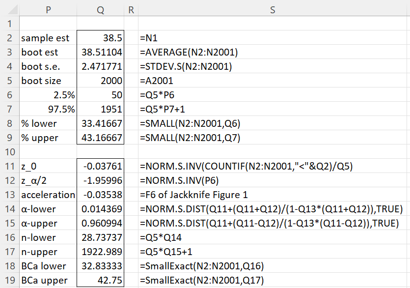
Figure 2 – Confidence intervals
We use the Real Statistics SMALLExact function in cells Q18 and Q19 since the values in cells Q16 and Q17 are not whole numbers. Since the 28th and 29th smallest bootstrap means are equal, we could have used the Excel SMALL function instead of SMALLExact. Similarly, we could have used the SMALL function in cell Q19 since the 1922nd and 1923th smallest bootstrap means are equal.
As stated above, the sample data is approximately normally distributed, and so we expect that the confidence interval will take the form x-bar ± se⋅ crit. This confidence interval, (33.50597, 43.49403), is shown in range V6:V7 of Figure 3 and is pretty similar to the percentile confidence interval described previously. The BCa confidence interval probably better reflects the skewness of the sample data (skewness = -.84475).
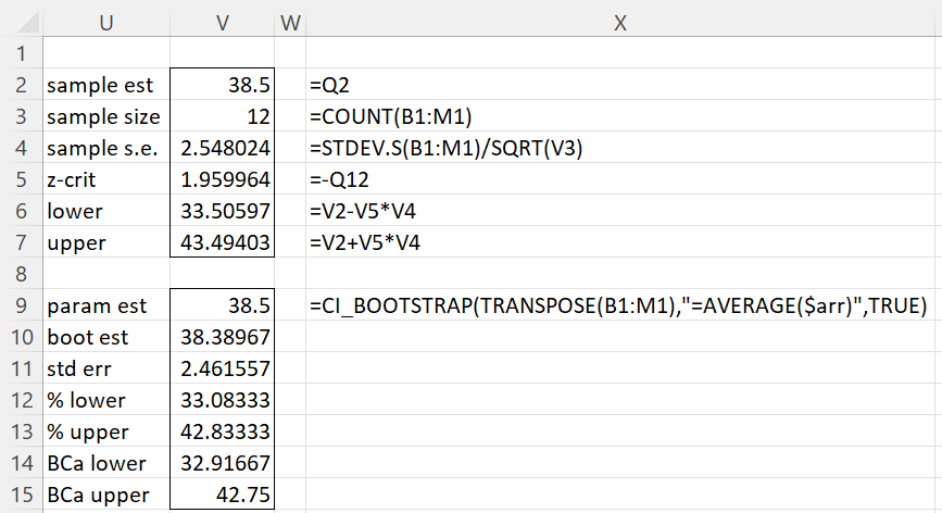
Figure 3 – More confidence intervals
We can also use the CI_BOOTSTRAP function to calculate both the percentile and BCa confidence intervals, as shown in the lower part of Figure 3.
One final note. We observe that the bootstrap mean shown in Figure 2 is 0.01104 higher than the sample mean. This could motivate us to shift the percentile confidence interval 0.01104 units to the left, obtaining the interval (33.40563,43.15563). It is unclear whether this is a better estimate, but some may recommend this adjustment.
Correlation Example
Example 2: Use bootstrapping to estimate the 95% confidence of the population correlation coefficient based on the sample of size 8 in range B2:C9 of Figure 2 of Jackknife (Example 2 of that webpage).
We use the lambda formula
=CI_BOOTSTRAP(B2:C9,”=CORREL(INDEX($arr,,1),INDEX($arr,,2))”,TRUE)
to obtain the results shown in Figure 4.
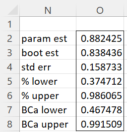
Figure 4 – Bootstrap confidence intervals for correlation
Examples Workbook
Click here to download the Excel workbook with the examples described on this webpage.
Links
References
DiCiccio, T. J., Efron, B. (1996) Bootstrap confidence intervals.
http://staff.ustc.edu.cn/~zwp/teach/Stat-Comp/Efron_Bootstrap_CIs.pdf
Efron, B., Tibshirani, R. J., (1993) An introduction to the bootstrap. Springer
https://books.google.it/books?hl=en&lr=&id=gLlpIUxRntoC&oi=fnd&pg=PR14&dq=Efron,+B.,+Tibshirani,+R.+J.,+(1993)+An+introduction+to+the+bootstrap.+Springer&ots=AaBr-7Kcy0&sig=M1FW6pzIvh1jgNfOXVKOE5G6uIk
Hello, Charles.
I have a question:
If I have a sample of pairs (xi, yi), i=1,2,…,n, and I use a least square linear regression model yi= bo+b1*xi+ei, where ei is the ith error of the model fitting and b0 and b1 are the parameters obtained, and I use a non parametric bootstrap (with replacement) B times for the pairs (xi, yi) for getting percentile confidence intervals for b0 and b1 (computing yij=b0j+b1j*xij, i=1,2,…,n; j=1,2,…,B),
is it a good aproximation to use the bootstrap percentile confidence interval as a prediction interval for a specific xp value: ypj=b0j+b1j*xp, or is needed a correction to convert the confidence interval to a prediction interval?
I Will be waiting for your answer.
Thank you very much.
Hello William,
The following may be helpful:
https://stats.stackexchange.com/questions/226565/bootstrap-prediction-interval
Charles