Resampling procedures are based on the assumption that the underlying population distribution is the same as a given sample. The approach is to create a large number of samples from this pseudo-population using the techniques described in Sampling and then draw conclusions based on some statistic (the mean, median, etc.) from this sample.
Resampling is generally simple to implement and doesn’t require complicated formulas. Unlike parametric techniques, few assumptions are made (e.g. data doesn’t need to be normal, and samples don’t necessarily need to be large). Resampling is useful when the population distribution is unknown or other techniques are not available.
We consider two types of resampling procedures: bootstrapping, where sampling is done with replacement, and permutation (also known as randomization tests), where sampling is done without replacement. Generally, bootstrapping is used for determining confidence intervals of some parameter, while randomization is used for hypothesis testing.
One sample case
Suppose we would like to calculate a confidence interval for the median. Since there are no standard statistical tests for such confidence intervals, we approach the problem via bootstrapping as described in the following example.
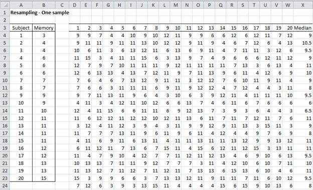
Example 1: Calculate a 95% confidence interval around the median for the memory loss program described in Example 1 of the Sign Test, but with the data given in columns A and B of Figure 1.
Figure 1 – Resampling – One-sample case
The sample has a mean of 9 and a median of 9.5.
Approach
We treat the sample as the population and draw 2,000 samples of size 20 (the same size as the original sample) with replacement. Referring to Figure 1, range D4:W4 represents the first sample, D5:W5 the second, etc. Each element in each sample is selected using the following function:
=INDEX(B4:B23,RANDBETWEEN(1,20))
We now take the median of each of the 2,000 samples (only the first 21 samples are shown in Figure 1). E.g. cell X4 contains the formula =MEDIAN(D4:W4). Next, we plot the distribution of the medians (i.e. range X4:X2003) in a histogram using Excel’s Histogram data analysis tool (or Excel’s charting capability), augmented with percentage and cumulative % columns. The results are shown in Figure 2.
Figure 2 – Analysis for Example 1
The value at the 2.5% percentile is 7, and the value at the 97.5% percentile is 10. Thus, we can consider the confidence interval as [7, 11], which contains the sample median of 9.5.
Observation
Instead of using the worksheet formula =INDEX(B4:B23,RANDBETWEEN(1,20)), we could use the formula RANDOMIZE(B4:B23) based on the Real Statistics array function RANDOMIZE to select a sample of 20 data elements with replacement.
Two independent samples
We now consider the case where there are two independent samples. When the data is normally distributed, we would typically use the t-test (for independent samples with equal variances or with unequal variances). Alternatives include the Wilcoxon Rank Sum or Mann-Whitney non-parametric test. We now show how to perform two independent sample testing using the permutation version of resampling.
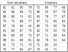
Example 2: Using resampling, determine whether there is a significant difference between the median life expectancy of smokers and non-smokers using the data described in Figure 3 (this is Example 3 from the Wilcoxon Rank Sum Test).
Figure 3 – Data for Example 2
Note that the median score of the non-smokers is 76.5 while the median score of smokers is 70.5, a difference of 6.
The null hypothesis is that there is no difference between the two groups, i.e.
H0: the median scores for the population of smokers and non-smokers are the same.
Approach
Based on the null hypothesis, we can assume that we have a single population of 78 (represented by the combined sample of 38 smokers and 40 non-smokers). To test the hypothesis, we take 2,000 random samples of size 78 from this population without replacement, and assume that for each sample the first 40 scores come from the non-smokers and the remaining 38 come from the smokers.
To draw these samples, we use the approach described in Sampling, namely, we use formulas of the form
=INDEX(J4:CI4,1,RANK(DC6,DC6:GB6))
where the range J4:CI4 contains all 78 data elements in the “population” and DC6:GB6 contains 78 random numbers, generated using RAND(). For each of the 2,000 samples, we calculate the median of the non-smokers and smokers and record the difference. A histogram of these median differences is provided in Figure 4.
Figure 4 – Resampling for two independent samples
Results
Now we need to check whether the mean difference of the original sample is in the extreme 5% of the total of the left and right tails of the sampling frequency table (2-tailed test). From Figure 4, we see that 1.60% of the samples have a median difference of -6 or less, and 4.90% of the samples have a median difference of 6 or more, for a total of 6.50%. This means that the probability of getting a sample in either tail based on the null hypothesis is .065 > .05 = α, and so we cannot reject the null hypothesis and cannot conclude with 95% confidence that there is a significant difference between the life expectancy of smokers and non-smokers.
Observations
If we had used a one-tailed test, then p-value = .049 < .05 = α, and so we would just barely reject the null hypothesis.
In the previous example, we chose to test the median. Using the same technique, we could have chosen to test the mean instead.
Instead of using the worksheet formula =INDEX(J4:CI4,1,RANK(DC6,DC6:GB6))), we could use the formula SHUFFLE(J4:CI4) based on the Real Statistics array function SHUFFLE to select a sample from the original 78 data elements without replacement.
Two matched samples
We now consider the case where we have two matched samples. When the data is normally distributed (or at least symmetric), we would use the Paired Sample t-test. Even for non-normal data, we can use the Wilcoxon Signed-Ranks non-parametric test. We now show how to address such problems using resampling techniques.
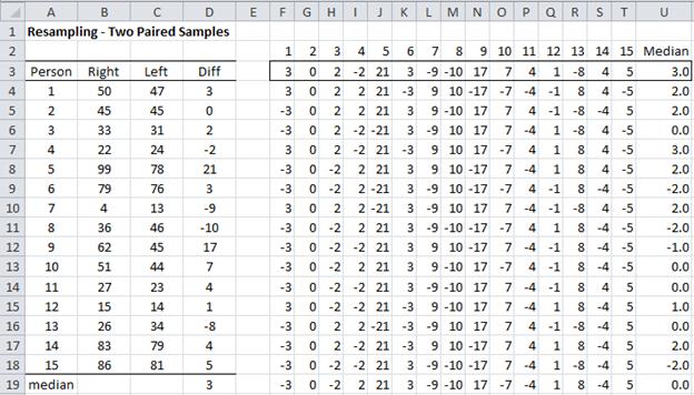
Example 3: Using resampling, determine whether there is a significant difference between the median life expectancy of smokers and non-smokers using the data described in Figure 3 (this is Example 1 from the Wilcoxon Signed-Ranks Test for Paired Samples)
The null hypothesis is there is no difference between a person’s ability to identify objects with their right eye from their ability with their left eye, i.e. the median difference is zero. As we have seen previously the data is skewed and so it might be better not to use the t-test. We will use resampling and assume that the population is as in the sample.
Approach
If the null hypothesis is true, then each of the 15 scores for the right eye is just as likely to be larger as smaller than the scores for their left eye, and so we can randomly exchange the scores of each person’s eyes. This is equivalent to randomly changing the sign of the difference between the scores. Thus, we take 2,000 samples each of size 15 (the size of the sample) using the sample data but randomly assigning the sign of the difference as positive or negative (with a 50% probability of each outcome).
This is a form of sampling without replacement. The absolute values of the elements in each sample are as in the population, only the signs vary.
Figure 5 – Resampling for paired samples
Figure 5 shows the first 16 samples (out of 2,000). The range F3:T3 contains the differences between the original data for the first sample. Each of the 15 data elements in the first sample is generated using the formulas
IF(RANDBETWEEN(0,1)=0,F$3,-F$3) through
IF(RANDBETWEEN(0,1)=0,T$3,-T$3)
and similarly for the other 1,999 samples. For each sample, we calculate the median and create a histogram of the 2,000 median values as shown in Figure 6.
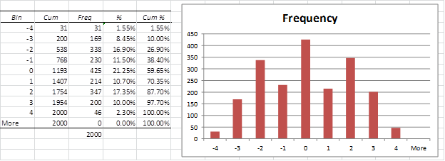
Figure 6 – Analysis for Example 3
The median of the original sample (i.e. the resampling “population”) is MEDIAN(D4:D18) = 3. From Figure 6, we see that 10.00% of all the samples have a median ≤ -3 and 12.30% have a median ≥ 3. Since 10.00 + 12.30% = 22.30% ≥ 5% = α, we cannot reject the null hypothesis, and so conclude there is no significant difference between the right and left eye of people in the population.
Additional Information
We use resampling techniques in a number of other places on this website. For example, see the following
- Resampling for Correlation
- Resampling for ANOVA
- Bootstrapping for Order Statistics
- Distribution Fitting Confidence Intervals
Click here for information about Real Statistics’ Resampling Data Analysis Tool.
Examples Workbook
Click here to download the Excel workbook with the examples described on this webpage.
Links
References
Howell, D. C. (2010) Statistical methods for psychology (7th ed.). Wadsworth, Cengage Learning.
https://labs.la.utexas.edu/gilden/files/2016/05/Statistics-Text.pdf
Efron, B. and Tibshirani, R. J. (1993) An introduction to the bootstrap. Springer


Hi Charles, I have the following two questions if you do not mind:
1. What i the difference between Monte Carlo Simulation and Bootstrapping? The web information are quite vague.
2. I am trying to estimate an extreme value based on sample measurements. I have tried to fit it to Weibull distribution (based on literature) and I got the parameters. Now I want to know the maximum value. Can I do that using bootstrapping without fitting it to Weibull distribution? and what equation to use to calculate the maximum in this case? because as I got from the reading is that bootstrapping can only be used for normal statistics not extreme values.
1. Monte Carlo Simulation is a general approach where you generate a random sample using a random number generator. This is commonly used to determine some property when an analytic approach is not available. E.g. to find the mean of some known distribution, you can generate 10,000 values that come from this distribution, take the mean of the sample and use this as an estimate for the mean of the distribution. See
https://www.real-statistics.com/sampling-distributions/simulation/
2. Bootstrapping is a particular approach that uses Monte Carlo Simulation. Additional information about bootstrapping can be found at
https://www.real-statistics.com/non-parametric-tests/resampling-data-analysis-tool/
The Real Statistics website contains a lot of information about extreme values that may be helpful. See
https://www.real-statistics.com/other-key-distributions/generalized-extreme-value-distribution/
https://www.real-statistics.com/distribution-fitting/method-of-moments/method-of-moments-gev-distribution/
https://www.real-statistics.com/distribution-fitting/distribution-fitting-via-maximum-likelihood/fitting-gev-distribution-mle/
Charles
Hi Charles,
Thanks so much for putting together these resources, truly appreciated. I had a quick question about the examples above. For calculating the p-value, where did the values 6 and 3 come from for examples 2 and 3 respectively?
For example 2, I imagine the 6 to come from the difference between the median score of the non-smokers (76.5) and the median score of smokers (70.5). But what about the 3 in example 3?
In general, do you take the value of the difference between the 2 original samples to calculate the p-value for the resampled data?
Thanks!
Hello Bob,
For Example 2, the answer to your questions is “yes”. You take the difference between the medians. This is the situation for comparing two independent samples
For Example, we are using a paired test; i.e. the samples are not independent of each other. In this case, you look at the differences between each of the pairs and take the median of these values. The comparison is usually this value (3 in this example) and zero.
Charles
Dear Charles,
Excellent tool. Thank you very much for designing it.
I have a query regarding the bins in the resampling procedure.
I have 10 scores: 8; 7.4; 7.7; 9; 9.2;6.9; 6.9; 7.8; 9; 9.2 (mean=8.11)
When I do resampling, one sample, mean, bootstrap, Min Bin=5, Max Bin=10, Bin Size=0.1, I get the following results:
bin freq
5 0
5.1 0
5.2 0
5.3 704
5.4 1296
5.5 0
More 0
It does not make any sense to me that, given the mean, I get all results in the 5 bins. Did I specify anything wrong?
I’m working with Windows 10, Excel 2010.
Best regards,
I don’t understand why in Figure 4, the median difference of 6 or more is 2.35%. As I see in histogram table, it should be 4.9% then the null hypothesis could not be rejected.
Please clarify this for me. Thank you.
Huyen,
Yes, you are correct. I believe that the 2.35% value was left over from a previous version of the data. In any case, I have now corrected the analysis on the webpage. Thank you very much for catching this error, thereby improving the accuracy of the website and making it easier for people to understand the statistical concepts being described. I really appreciate your help.
Charles
Thanks Charles. This is a great resource (examples are so much better than working through textbook equations!). I will dive into doing some confidence intervals for Gini Coefficients!
Dear Charles,
Your website has proven an invaluable resource–thank you for creating it!
I have a dataset that is both moderately skewed and heteroskedastic, so I am using your (Randomization) Resampling method. My data are proportions, so values are between 0-1.
In the output from the Resampling procedure, a large percentage (~40%) of the bins generated are outside the upper boundary of my dataset–that is, they are greater than 1. Is this a problem for the validity of the F-stat included in the output?
If I understand how resampling works, it seems I’m comparing the observed data distributions (of my three groups) to a “population” distribution generated on the basis of my dataset. On the surface, it seems conceptually odd that I would compare distributions whose values are between 0-1 to distributions that have a much greater range (about 0-5, from what I can tell), especially since 1 represents ceiling performance on my task.
I appreciate any help you can provide,
Emily
Emily,
I don’t quite understand why any of the bins would be outside the range 0 to 1.
If you send me an Excel file with your data and the analysis that you did, I will try to figure what is going on.
You can find my email address at Contact Us.
Charle
Charles,
I sent a sample of the data and the analyses earlier today–looking forward to your feedback!
Emily
Excellent tutorial!
Can you use this technique to calculate confidence intervals for proportions, i.e. polling studies where the sample size is small? Thank you…
Yes
Very interesting and helpful…
Can you use this technique to determine confidence intervals for binomially distributed proportions, i.e. polling studies with small samples? Thanks…
Yes
Thanks for your tutorial!!
I am also trying to use the bootstrapping approach to evaluate field significance for trend test detection (e.g. Mann-Kendall test) in hydro-climatic extremes analysis. Can you please advise me on this matter?
Your help is highly appreciated. Thanks.
I have not yet provided a bootstrapping version of Kendall’s test. You will need to do this yourself.
The testing of Kendall’s correlation coefficient is described on the website as is bootstrapping. Obviously you will need to duplicate the bootstrapping approach used for other tests for the Kendall’s test.
Charles
Many thanks for your explanation.
Sorry that I couldn’t help you further.
Charles
This is extremely helpful!!! I am currently considering using bootstrapping to apply a lineal correlation model between two variables. Do you have any suggestions as to how to do it? Thanks!
Malena,
See the following webpage:
Resampling for Correlation
Charles