We can also use simulation to estimate the p-values of the Mann-Whitney test. This approach will yield approximate values. Accuracy increases as the number of simulations is increased. Also, ties are taken into account.
Example
Example 1: Determine the approximate p-value for the Mann-Whitney test on the data in range A3:B8 of Figure 1 using simulation.
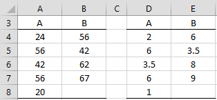
Figure 1 – Mann-Whitney data
The right side of Figure 1 contains the ranks of the data on the left side. We now perform 20 simulations of randomized permutations of these rankings into two groups: the larger group with 5 elements, followed by the group with 4 elements.
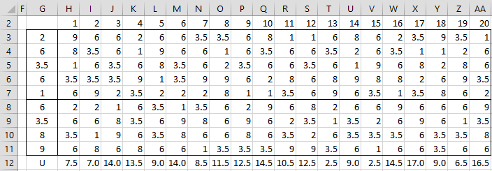
Figure 2 – Mann-Whitney simulation
For example, we use the Real Statistics formula =SHUFFLE(G3:G11) to output in range H3:H11. The U value is equal to the sum of the ranks for the smaller random sample minus the minimum such sum, namely 4(4+1)/2 = 10. Thus, the U value for the first random sample (cell H12) is 7.5 as calculated by the formula =SUM(H8:H11)-10. The other 19 random values for U are calculated in the same way.
Note that the U for the original sample is 3.5, as calculated by =MANN(A4:A8,B4:B8). 1 of the 20 randomly generated a U value in Figure 2 less than or equal to 3.5 (namely, sample 13). Thus, an estimate of the p-value of the one-tailed Mann-Whitney test (based on the left tail) is p-value = 1/20 = .05. If the right tail is used, we need to look for the number of samples with a U value of 16.5 or higher. Here 16.5 is calculated by 4∙5 – 3.5 = 16.5. This time, there are 2 such values (from samples 17 and 20), and so the right-tailed test also has a p-value of .10. The two-tailed test therefore has a p-value of .05 + .10 = .15.
Increasing the number of simulations
Since the number of iterations in the simulation is very small, these estimated p-values are not very accurate. If, instead, we perform 10,000 simulations, we get the results shown in Figure 3.

Figure 3 – Mann-Whitney simulation based on 10,000 samples
The left side shows the number of times each potential U value between 0 and 20 occurs in the 10,000 iterations. The right side shows the cumulative distribution based on this simulation. E.g. the probability of U is .0574, as calculated by the formula =AJ7+AD8/10000 in cell AJ8.
Thus, the p-value for U is (88+486)/10000 = .0574 (left-tailed test), which is the same as the value in cell AJ10. The p-value for U is (496+91+244)/10000 = .0831 (right-tailed test), which is the same as the value calculated by the formula =1-AM15. Finally, the p-value of the two-tailed test is, therefore, .0574+.0831 = .1405. None of these results is significant for α = .05.
Worksheet Function
Real Statistics Function: The Real Statistics Pack also provides the following array function for the samples in R1 and R2, where iter is the number of simulations.
MW_SIMUL(R1, R2, lab, iter): returns a column array with the U statistic for R1 and R2, i.e. U = MANN(R1,R2), the p-value for the left-tailed test of, the p-value for the right-tailed test and the p-value for the two-tailed test; if lab = TRUE (default FALSE) then an extra column of labels is appended to the output.
For Example 1, the output of MW_SIMUL(A4:A8, B4:B8, TRUE) is shown in Figure 4.
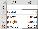
Figure 4 – Output from MW_SIMUL
Links
References
Howell, D. C. (2010) Statistical methods for psychology (7th ed.). Wadsworth, Cengage Learning.
https://labs.la.utexas.edu/gilden/files/2016/05/Statistics-Text.pdf
Zar. J. H. (2010) Biostatistical analysis 5th Ed. Pearson