Basic Concepts
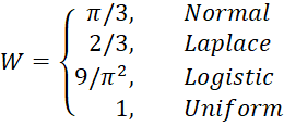
To estimate the power of a Mann-Whitney (or Wilcoxon Rank-Sum) test for two samples of sizes n1 and n2, first calculate the adjusted sample sizes n1* = n1/W and n2* = n2/W, where W depends on the distribution of the sample as follows
Then, conduct a two independent sample t-test with equal variances using the adjusted sample sizes n1* and n2*.
Another approach is to use simulation. In this approach, two samples are generated based on selected criteria (distribution, sample sizes, and effect sizes). The Mann-Whitney test is then performed on these samples to determine whether or not there is a significant result (based on a selected significance level alpha).
If a large number of such samples are generated at random, we can determine what percentage of these samples yield a significant result. This percentage is an estimate for the power of the MW test.
E.g. for a simulation where both samples come from a normal distribution, we can assume that the standard error is 1, and so the effect size for each sample is simply the mean. In general, for any distribution, we will assume that the second parameter is 1, and so the effect size is equal to the value of the first parameter.
Example
Example 1: Use simulation to determine the power of the MW test for two samples of size 10 with effect sizes 1 and 2.
In Figure 1, we show the results from 20 such simulations. To accomplish this, we place the formula =NORM.INV(RAND(),1,1) in cell A2, highlight range A2: T11, and press Ctrl-R and Ctrl-D. This produces 20 random samples with an effect size of 1. Similarly, we place =NORM.INV(RAND(),2,1) in cell A12, highlight range A12:T21, and press Ctrl-R and Ctrl-D. This produces 20 samples with an effect size of 2.

Figure 1 – 20 MW simulations
We now calculate the p-value of each of the 20 MW tests by inserting the formula =MWTEST(A2:A11,A12:A21) in cell A22, highlighting range A22:T22, and pressing Ctrl-R. We see from row 23 that 11 of the 20 tests were significant, yielding an estimated power of 55%.
Worksheet Function
Real Statistics Function: The following function is provided in the Real Statistics Pack.
MW_POWER(effect1, effect2, n1, n2, iter, dist, tails, ties, cont, alpha) = the power of a Mann-Whitney test on two samples from a distribution of type dist (default “norm”) of sizes n1 and n2 with corresponding effect sizes effect1 and effect2 based on a simulation with iter iterations (default 100).
tails = # of tails = 1 or 2 (default). If ties = TRUE (default), a ties correction is applied. If cont = TRUE (default), a continuity correction is applied. alpha = the significance level (default .05). The supported distributions and the corresponding dist argument are as shown in Figure 2.

Figure 2 – dist argument
Note that for these distributions, the effect size is equal to the mu parameter, assuming the second parameter is one.
We can use the MW_POWER function to provide a better estimate of the power of the MW test in Example 1. This is done by increasing the number of simulations from 20 to 10,000. We see from cell B9 of Figure 3 that the power is about 51.4%. Even with 10,000 iterations, this value is approximate since if repeated, the value may differ (although in the simulations that I have conducted, the value ranged between 51% and 52.5%).
Here, cell B9 contains the formula
=MW_POWER(B4,B5,B6,B7,B8,”norm”,2,TRUE,TRUE,0.05)

Figure 3 – Power of a MW test
Power of an equivalent t-test
The power of an equivalent two-sample t-test, i.e. two samples of size 10 and an effect size = (2-1)/1 = 2 is 56.2 as calculated by the formula =T2_POWER(1,10,10). Note that if we change the sample sizes from 10 to 10/(π/3), using the approximation for the MW test described earlier, we obtain power of T2_POWER(1,10*3/Pi(),10*3/Pi()) = 54.0%, which is similar to the value calculated above.
To find the sample sizes required to obtain statistical power of 80%, we first note that samples of size 17 are required for the two-sample t-test, via the formula =T2_SIZE(1,.8). Since a little more is required for the MW test, we guess that samples of size 18 are required, which is confirmed by the result shown in column C of Figure 3. Note that samples of size 30 are required to achieve power of 95% (instead of 17 for the two-sample t-test).
Examples Workbook
Click here to download the Excel workbook with the examples described on this webpage.
Links
References
NCSS PASS (2011) Mann-Whitney U or Wilcoxon Rank-Sum tests for non-inferiority
https://www.ncss.com/wp-content/themes/ncss/pdf/Procedures/PASS/Mann-Whitney_U_or_Wilcoxon_Rank-Sum_Tests_for_Non-Inferiority.pdf
Al-Sunduqchi, Mahdi S. (1990) Determining the Appropriate Sample Size for Inferences Based on the Wilcoxon Statistics. Ph.D. dissertation under the direction of William C. Guenther, Dept. of Statistics, University of Wyoming, Laramie, Wyoming.