We now describe how to create a confidence interval for the difference between the population medians using the Hodges-Lehmann estimation.
Examples
Example 1: Find the 95% confidence interval for the difference between the population medians based on the data in Example 1 of Mann-Whitney Test (repeated in range A3:D18 of Figure 1).
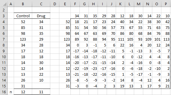
Figure 1 – Set-up for calculating the confidence interval
There are 12 elements in the Control sample (range B4:B15) and 11 elements in the Drug sample (range C4:C14). Thus, there are 12∙11= 132 pairs of elements from both samples. All 132 possible differences are shown in range F4:P15. For example, the difference between the first Control element (cell B4) and the second Drug element (cell C5) is 52 – 31 = 21, shown in cell G4, as calculated by the formula =$E4-G$3. Note that the range F3:P3 contains the array formula =TRANSPOSE(C4:C14).
Calculations
Using the MWDIST and MWINV functions, we see that the two-tailed critical value for α = .05 when the sample sizes are 11 and 12 is 33. Thus, we have the analysis shown in Figure 2.
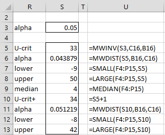
Figure 2 – Calculation of the confidence interval
The 95% confidence interval is bounded by the 33rd smallest and 33rd largest values in range F4:P15, as calculated in cells S7 and S8. The result is a 95% confidence interval of [-9, 50].
Hodges-Lehmann Median
The median of all the values in range F4:P15, called the Hodges-Lehmann median, is 4 (cell S9). This can be used as an alternative effect size measurement.
Range S10:S13 is similar to range S5:S8, except that the confidence interval calculated is based on the critical value shown in cell S5 plus 1 (as shown in cell S10). Cell S11 shows the approximate alpha value corresponding to the value in cell S10. This means that the 94.45% confidence interval is [-8, 42], where 94.45% = 1 – .05556.
Another Example
Example 2: Find the 95% confidence interval for the difference between the population medians based on the data in Example 2 of Mann-Whitney Test (repeated in range A3:H13 of Figure 3).
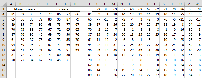
Figure 3 – Set up for Mann-Whitney confidence interval
Just as we did for Example 1, we create a table of differences. Since there are 40 non-smokers and 38 smokers, this is a 40 × 38 table occupying the range K4:AV43 of Figure 3 (with only the upper left side of the table visible).
Since the sample sizes are larger than those included in the table of critical values, we use the normal approximation, i.e. the ranks of the lower and upper bounds of the confidence interval are
![]()
where zcrit = the critical value for the standard normal distribution for α/2 = .025.
Figure 4 displays the calculations required to obtain the 95% confidence interval and a Hodges-Lehmann median of 7. We see from the figure that there is a 95.11% confidence interval of [2, 13] and a 94.99% confidence interval also of [2, 13]. Since both intervals are the same, we conclude that the 95% confidence interval is indeed [2, 13].
This won’t always be the case. In general, we will find that the alpha value for the first confidence interval will be at most .05, while the alpha value for the second will be a little larger than .05, and so we will have two confidence intervals, one a little more than 95% and one a little less than 95%.
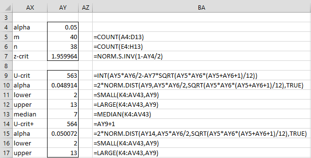
Figure 4 – Calculation of the confidence interval
Worksheet Function
Real Statistics Function: The Real Statistics Pack provides the following array function to calculate the confidence interval based on the samples in R1 and R2, where the significance level is the α value (default .05).
MW_CONF(R1, R2, lab, type, alpha): returns a 9 × 1 column array with the lower and upper bounds of the 1 – alpha confidence interval and the Hodges-Lehmann median. If lab = TRUE (default FALSE), then an extra column with labels is included in the output. When type = 0 (default), then the normal approximation is used. Finally, if type = 1, then the exact test is used.
For Example 1, the array formula =MW_CONF(B4:B15,C4:C15,TRUE,1) returns the values shown in range R5:S13 of Figure 2. For Example 2, the array formula =MW_CONF(A4:D13,E4:H13,TRUE) returns the values in range AX9:AX17 of Figure 4.
As we have seen in Example 2, with an integer critical value, it is not always possible to achieve a confidence interval of exactly 1–α. For this reason, the MW_CONF generates two confidence intervals. The first corresponds to an alpha value that is at most α, while the second corresponds to the smallest significance level that is larger than α.
Examples Workbook
Click here to download the Excel workbook with the examples described on this webpage.
Links
References
SAS (2019) Hodges-Lehmann estimation of location shift
https://documentation.sas.com/doc/en/statug/15.2/statug_npar1way_details19.htm
Hollander, M., Wolfe, D. A. (1999) Nonparametric statistical methods, 2nd ed. Wiley
Influential Points (2015) The Wilcoxon-Mann-Whitney test
https://influentialpoints.com/Training/wilcoxon-mann-whitney_u_test-principles-properties-assumptions.htm
Hi Charles,
Thank you so much for this excellent and informative website.
I have calculated a confidence interval with MW_CONF as [-22,-7]
How do I represent this interval as actual data values, rather than the rank values?
Would I be correct in using the data values with ranks |-7| = 7 and |-22| = 22?
This would then give me a larger Lower Confidence Interval Value than my Upper Confidence Interval Value.
For clarity, the data value with rank 7 = 36.849 and the data value with rank 22 = 40.896.
Hi Matt,
I believe that the confidence intervals refer to the actual data values and not the ranks in this case. Here the data values are the potential differences between the medians.
Charles
Hello!
Thanks for the great explanation and accompanying download,
It seems the software blocks the user from making changes to the array – was there a version that allowed this?
Additionally, I’m wondering if there’s a method that makes it easy to add many n’s (using imputed data so a few thousand values to add!)
Many thanks – a confused thesis student 🙂
Hello Sarah,
Glad that the explanation was helpful.
1. You say that the software blocks changes to the array. Which array are you referencing. Generally, Excel blocks changes to an array that is produced by a function, and so this may be the problem. THis can be overcome for Excel 365 users.
2. Adding n’s: I don’t know what you are referencing by n’s. Are you referencing missing data? Can you give me an example?
Charles
Thanks for your respones Charles!
I have given it a go both on onedrive excel and on the laptop app for office 365. Essentially I have imputed data, so each of my categories has 1500+ data entries (e.g., for one n=1684). When I go to increase how much data is transposed in the chart on CI 1 (changing “=TRANSPOSE(C4:C14)” to “=TRANSPOSE(C4:C1687)”, it says I can’t change any part of the array. Maybe my software is just not compatible, but any thoughts you had on how to overcome this would be greatly appreciated!
Hello Sarah,
Without seeing all the details, I am not able to completely answer your question. Let me address the part that is clear to me.
1. Suppose that you have placed the array formula =TRANSPOSE(C4:C14) in range E1:K1. To increase the size you need to highlight the range E1:BLZ1, insert the formula =TRANSPOSE(C4:C1687), and press Ctrl-Shft-Enter.
2. Since you are using Excel 365, the simpler approach is to highlight range E1:K1 and press the Cancel key to erase the =TRANSPOSE(C4:C14) array formula. Now place the formula =TRANSPOSE(C4:C1687) in cell E1 and press Enter. The dynamic array capability of Excel 365 should do the rest for you automatically.
Charles
Kia ora Charles,
Brilliant, thanks for that explanation!
The data points in the first few sections now seem to all be arranged without issue and the array is able to be edited.
I have the Real Statistics add-in installed, but still seem to be having issues with the formulas in the calculations section. They are all changed to properly reflect my datapoints (e.g., U-crit with =@MWINV(BMC3,C4913,B4913)), but all values except the median have the error “#NAME?”. Not sure why they’re not computing?
Apologies for the confusion, and thanks for all your help, it really is appreciated!
Sarah
HI Sarah,
What do you see when you enter the formula =VER() in any cell?
Charles
Same thing – when I enter =VER() I get #NAME?
Hi Sarah,
This means that you haven’t installed the Real Statistics software. The #NAME? errors will go away once you have installed the software.
See https://real-statistics.com/free-download/real-statistics-resource-pack/
Charles
Hi Charles,
Thank you very much for this page!
Unfortunately I don’t succeed in applying the array formula MW_CONF(R1, R2, lab, type, alpha) by using your dataset. Excel reports error codes (I already replaced ‘,’ by ‘;’). Is it perhaps impossible to generate Figure 2 (S5;S13) by only using the dataset from B4:B15 – C4:C14 and the array formula MW_CONF(R1, R2, lab, type, alpha)? Do I need to do more steps?
Thank you in advance!
Have you installed the free Real Statistics software (an add-in to Excel that gives you access to a lot of statistical capabilities in Excel)?
Charles
Dear Charles,
Thanks a lot for answering my question, I installed the Real Statistics software (Macbook) (the add-in is only visible when using ‘control + m’).
Something just came into my mind: Changing ‘FALSE’ into the translated equivalent and it worked!
Thank you very much for this document.
Kind regards,
Winne
Good to see that you got it to work.
Charles
Hi
I am so glad for this page and the add-in to excel .
I managed to do all the calculations except the =SMALL and =LARGE, in simply will not appear in the cell when i write it. The rest of my excel is in danish, do you think that could be an issue? or do you have any suggestions for me?
Best regards Johanne 🙂
Hi Johanne,
The SMALL and LARGE functions are called MINDSTE and STØRSTE in the Danish version of Excel.
You can find a list of the Danish names of the standard Excel functions at https://www.perfectxl.com/excel-glossary/what-is-excel-function/translations-english-danish/
There are no substitute names for Real Statistics functions. These should work in any version of Excel.
Charles
Can u please help with a manual computations for Mann Whitney confidence interval, thank uu
This webpage is intended to show how to do this. What sort of questions about this do you have?
Charles
Hi Charles,
When using the formula MW_CONF(R1, R2, lab, type, alpha) I only get the U-crit, not the rest of the expected output. I use Excel 2013. Do you have any idea what the problem might be?
Hi Mats,
MW_CONF is an array function and so it returns a range of cells, but you must use it in a slightly different way. This is a standard feature of Excel. See the following webpage for more details:
Array Formulas and Functions
Charles
Thank you for a rapid reply that solved my problem!
How can i like this post hundreds of times? T’ve seeked for weeks for this. Huge help.
Long live Charles
Hi Charles,
This is a really great site you have developed here. I have downloaded the Real statistics add in and tested it with your example above – it is working fine. I cannot seem to work it through with my own data though. The problem seems to be with datasets that are larger than about 15 samples in each of 2 groups. Is there a workaround or do you have plans to update the add in to allow for larger sample sizes?
Eileen,
Yes, there is another approach which I am about to add to the website. It will work for any size samples.
Charles
Eileen,
I have now revised this webpage. The new approach will work for any size samples. Shortly, I will issue a new version of the Real Statistics software which will implement this approach.
Charles
That seems great, exactly what I need. Do you happen to have the excel workbook for that? I have some trouble doing the ‘by pairing the kth value in R4:R135 with the kth value’…
Thank you so much!
Sorry, I got this… thanks!