FGLS Method for Autocorrelation

Introduction

The GLS approach to linear regression requires that we know the value of the correlation coefficient ρ. Unfortunately, usually, we don’t know the value of ρ, although we can try to estimate it from sample values. Since we are using an estimate of ρ, the approach used is known as the feasible generalized least squares (FGLS) or estimated generalized least squares (EGLS).

Using the Durbin-Watson coefficient

The sample autocorrelation coefficient r is the correlation between the sample estimates of the residuals e₁, e₂, …, e_n-1 and e₂, e₃, …, e_n. Since E[e_i] = 0 (even if there is autocorrelation), it follows that

Actually, in the case of autocorrelation, we will use the slightly modified definition

Note that the Durbin-Watson coefficient can be expressed as

and so

d ≈ 2(1 – r)

Thus, we can estimate ρ by r ≈ 1 – d/2.

Example

Example 1: Use the FGLS approach to correct the autocorrelation in Example 1 of Durbin-Watson Test (the data and calculation of residuals and Durbin-Watson’s d are repeated in Figure 1).

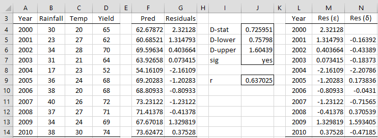
Figure 1 – Estimating ρ from Durbin-Watson d

We estimate ρ from the sample correlation r (cell J9) using the formula =1-J4/2. The δ residuals are shown in column N. E.g. δ₂ (cell N5) is calculated by the formula =M5-M4*J$9. We see from Figure 2 that, as expected, the δ are more random than the ε residuals since presumably the autocorrelation has been eliminated or at least reduced.

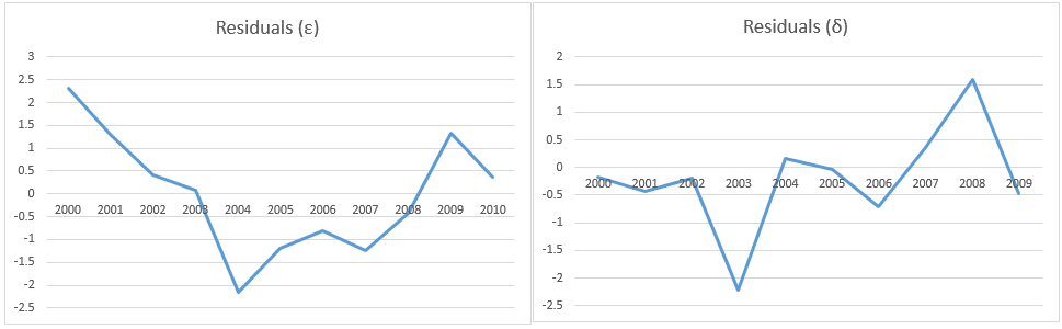
Figure 2 – Comparison of the residuals

We now calculate the generalized difference equation as defined in GLS Method for Addressing Autocorrelation.

where

and ρ = .637 as calculated in Figure 1. This form of OLS regression is shown in Figure 3.

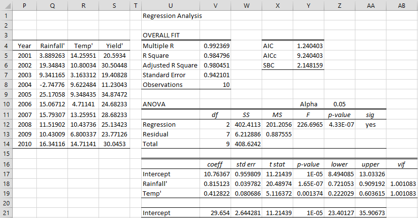
Figure 3 – FGLS regression using Durbin-Watson to estimate ρ

We place the formula =B5-$J$9*B4 in cell Q5, highlight the range Q5:S14, and press Ctrl-R and Ctrl-D to fill in the rest of the values in columns Q, R, and S. We now perform linear regression using Q3:R14 as the X range and S3:S14 as the Y range. The result is shown on the right side of Figure 3.

.8151 (cell V18) is the regression coefficient for Rainfall′ but also for Rainfall, and .4128 (cell V19) is the regression coefficient for Temp′ and also for Temp. The Intercept coefficient has to be modified, as shown in cell V21 using the formula =V17/(1-J9).

Note that the three regression coefficients (29.654, .8151, .4128) are a little different from the incorrect coefficients (30.058, .7663, .4815) calculated by the original OLS regression (calculation not shown). Similarly, the standard errors of the FGLS regression coefficients are 2.644, .0398, .0807 instead of the incorrect values 3.785, .0683, .1427.

Observations

The FGLS standard errors are generally higher than the originally calculated OLS standard errors, although this is not always the case, as we can see from this example.

If had used the Prais-Winsten transformation for 2000, then we would have obtained regression coefficients 16.347, .9853, .7878 and standard errors of 10.558, .1633, .3271. This time the standard errors would have been larger than the original OLS standard errors.

Although the results with and without the estimate for 2000 are quite different, this is probably due to the small sample, and won’t always be the case.

Using linear regression

We can also estimate ρ by using the linear regression model

ε_i = ρε_i-1 + δ_i

which is implemented using the sample residuals e_i to find an estimate for ρ using OLS regression.

Example

Example 2: Repeat Example 1 using the linear regression approach.

This time we perform linear regression without an intercept using H5:H14 as the X range and G5:G14 as the Y range. The slope parameter .4843 (cell K17) serves as the estimate of ρ.

Figure 4 – Estimating ρ via linear regression

From this point on, we proceed as in Example 1, as shown in Figure 5.

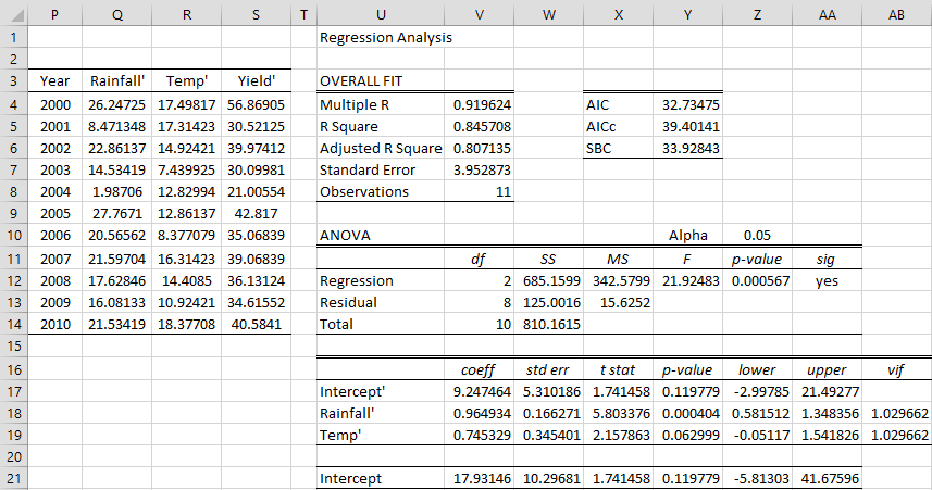
Figure 5 – FGLS regression including Prais-Winsten estimate

This time, we show the calculations using the Prais-Winsten transformation for the year 2000. The Rainfall′ for 2000 (cell Q4) is calculated by the formula =B4*SQRT(1-$K$17^2). Highlighting the range Q4:S4 and pressing Ctrl-R fills in the other values for 2000.

If no estimate for 2000 were used then the regression coefficients would be 29.124, .8107, .4441 with standard errors 2.715, .0430, .0888.

Observations

There is also an iterative version of the linear regression FGLS approach called Cochrane-Orcutt regression. See Cochrane-Orcutt Regression for more details

Until now we have assumed first-order autocorrelation, which is defined by what is called a first-order autoregressive AR(1) process, namely

ε_i = ρε_i-1 + δ_i

The linear regression methods described above (both the iterative and non-iterative versions) can also be applied to p-order autoregressive AR(p) processes, namely

ε_i = ρ₁ε_i-1 + ⋅⋅⋅ + ρ_pε_i–p + δ_i

References

Wooldridge, J. M. (2013) Introductory econometrics, a modern approach (5th Ed). Cengage Learning

Wikipedia (2018) Generalized least squares
https://en.wikipedia.org/wiki/Generalized_least_squares

Wikipedia (2018) Winsten estimation
https://en.wikipedia.org/wiki/Prais%E2%80%93Winsten_estimation