Measures of Central Tendency

Basic Concepts

We consider a random variable x and a data set S = {x₁, x₂, …, x_n} of size n which contains values for the random variable x. The data in S can represent either a population being studied or a sample drawn from such a population. We can also view the data as defining a distribution, as described in Discrete Probability Distributions.

We seek a single measure (i.e. a statistic) that somehow represents the center of the entire data set S. The commonly used measures of central tendency are the mean, median, and mode. Besides the normally studied mean (also called the arithmetic mean), we also consider two other types of mean: the geometric mean and the harmonic mean.

Worksheet Functions

Excel Functions: If R1 is an array or range that contains the data elements in S then the Excel formula that calculates each of these statistics is shown in Figure 1.

Figure 1 – Measures of central tendency

Handling non-numeric data

While formulas such as AVERAGE(R1) (as well as VAR(R1), STDEV(R1), etc. described on other webpages) ignore any empty or non-numeric cells, they return an error value if R1 contains an error value such as #NUM or #DIV/0!. This limitation can often be overcome by using one of the following array formulas:

=AVERAGE(IF(ISERROR(R1), ””, R1))

=AVERAGE(IFERROR(R1, ””)

These formulas return the mean of all the cells in R1 ignoring any cells that contain an error value. Since these are array formulas, you must press Ctrl-Shft-Enter (unless you are using Excel 365). An alternative approach is to use the Real Statistics DELErr function.

Worksheet Function

Real Statistics Function: The Real Statistics Resource Pack provides the following array function:

DELErr(R1) = the array of the same size and shape as R1 consisting of all the elements in R1 where any cells with an error value are replaced by a blank (i.e. an empty cell).

E.g. to find the average of the elements in an array R1 which may contain error values, you can use the formula

=AVERAGE(DELErr(R1))

In this case, you only need to press the Enter key and don’t have to press Ctrl-Shft-Enter.

Data Analysis Tool

Real Statistics Data Analysis Tool: The Remove error cells option of the Reformatting a Data Range data analysis tool described in Reformatting Tools makes a copy of the inputted range where all cells that contain error values are replaced by empty cells.

To use this capability, press Ctrl-m and double-click on Reformatting a Data Range. When the dialog box shown in Figure 2 of Reformatting Tools appears, fill in the Input Range, choose the Remove error cells option, and leave the # of Rows and # of Columns fields blank. The output will have the same size and shape as the input range.

Mean

We begin with the most commonly used measure of central tendency, the mean.

Definition 1: The mean (also called the arithmetic mean) of the data set S is defined by

Excel Function: The mean is calculated in Excel using the function AVERAGE.

Real Statistics Function: The mean can also be calculated using the Real Statistics function MEAN, which is equivalent to AVERAGE.

Example 1: The mean of S = {5, 2, -1, 3, 7, 5, 0, 2} is (2 + 5 – 1 + 3 + 7 + 5 + 0 + 2) / 8 = 2.875. We achieve the same result by using the formula =AVERAGE(C3:C10) in Figure 2.

Figure 2 – Excel examples of central tendency

When the data set S is a population the Greek letter µ is used for the mean. When S is a sample, then the symbol x̄ is used.

Frequency Tables

When data is expressed in the form of frequency tables then the following property is useful.

Property 1: If x̄ is the mean of sample {x₁, x₂, …, x_m} and ȳ is the mean of sample  {y₁, y₂, …, y_n} then the mean of the combined sample is

Similarly, if µ_x is the mean of population {x₁, x₂, …, x_m}  and µ_y is the mean of population {y₁, y₂, …, y_n} then the mean of the combined population is

Based on Property 1, the mean of the combined data in Data 1 and Data 2 from Figure 2 can be calculated as 3.4 using the formula =(B13*B15+D13*D15)/(B13+D13), which yields the same value as =AVERAGE(B4:B11,D4:D11).

Worksheet Functions

Real Statistics Functions: The Real Statistics Resource Pack furnishes the following array functions:

COUNTCOL(R1) = a row array that contains the number of numeric elements in each of the columns in R1

SUMCOL(R1) = a row array that contains the sums of the data elements in each of the columns in R1

MEANCOL(R1) = a row array that contains the means of each of the columns in R1

COUNTROW(R1) = a column array that contains the number of numeric elements in each of the rows in R1

SUMROW(R1) = a column array that contains the sums of the data elements in each of the rows in R1

MEANROW(R1) = a column array that contains the means of each of the rows in R1

Example 2: Use the COUNTCOL, SUMCOL, and MEANCOL functions to calculate the number of cells in each of the three columns in the range L4:N11 of Figure 3 as well as their means and sums.

Figure 3 – Count, Sum, and Mean by Column

The array formula =COUNTCOL(L4:N11) produces the first result (shown in range L13:N13), while the formula =MEANCOL(L4:N11) produces the second result (in range L14:N14) and the formula =SUMCOL(L4:N11) produces the third result (in range L15:N15).

Remember that after entering any of these formulas you must press Ctrl-Shft-Enter.

See Weighted Mean and Median for how to calculate the weighted mean.

Median

Definition 2: The median of the data set S is the middle value in S when the data is in sorted order. If you arrange the data in increasing order the middle value is the median. When S has an even number of elements there are two such values; the average of these two values is the median.

Excel Function: The median is calculated in Excel using the function MEDIAN.

Example 3: The median of S = {5, 2, -1, 3, 7, 5, 0} is 3 since 3 is the middle value (i.e. the 4th of 7 values) in -1, 0, 2, 3, 5, 5, 7. We achieve the same result by using the formula =MEDIAN(B3:B10) in Figure 2.

Note that each of the functions in Figure 2 ignores any non-numeric values, including blanks. Thus the value obtained for =MEDIAN(B3:B10) is the same as that for =MEDIAN(B3:B9).

The median of S = {5, 2, -1, 3, 7, 5, 0, 2} is 2.5 since 2.5 is the average of the two middle values (2 and 3) of -1, 0, 2, 2, 3, 5, 5, 7. This is the same result as =MEDIAN(C3:C10) shown in Figure 2.

See Weighted Mean and Median for how to calculate the weighted median.

Mode

Definition 3: The mode of the data set S is the value of the data element that occurs most often.

Example 4: The mode of S = {5, 2, -1, 3, 7, 5, 0} is 5 since 5 occurs twice, more than any other data element. This is the result we obtain from the formula =MODE(B3:B10) in cell B19 of Figure 2. When there is only one mode, as in this example, we say that S is unimodal.

If S = {5, 2, -1, 3, 7, 5, 0, 2}, the mode of S consists of both 2 and 5 since they each occur twice, more than any other data element. When there are two modes, as in this case, we say that S is bimodal.

Excel Function: The mode is calculated in Excel by the worksheet function MODE. If R1 contains unimodal data then MODE(R1) returns this unique mode. For the first data set in Example 3, this is 5. When R1 contains data with more than one mode, MODE(R1) returns the first of these modes. For the second data set in Example 4, this is 5 (since 5 occurs before 2, the other mode, in the data set). Thus MODE(C3:C10) = 5.

As remarked above, if there is more than one mode, MODE returns only the first, although if all the values occur only once then MODE returns an error value. This is the case for S = {5, 2, -1, 3, 7, 4, 0, 6}. Thus MODE(D3:D10) = #N/A.

Starting with Excel 2010 the array function MODE.MULT is provided which is useful for multimodal data by returning a vertical list of modes. When we highlight C19:C20 and enter the array formula =MODE.MULT(C3: C10) and then press Ctrl-Alt-Enter, we see that both modes are displayed.

The function MODE.SNGL is also provided with versions of Excel starting with Excel 2010. This function is equivalent to MODE.

Geometric Mean

Definition 4: The geometric mean of the data set S is calculated by

This statistic is commonly used to provide a measure of the average rate of growth as described in Example 5.

Example 5: Suppose the sales of a certain product grow 5% in the first two years and 10% in the next two years, what is the average rate of growth over the 4 years?

If sales in year 1 are $1 then sales at the end of the 4 years are (1 + .05)(1 + .05)(1 + .1)(1 + .1) = 1.334. The annual growth rate r is that amount such that (1+r)⁴ = 1.334. Thus r = 1.334^1/4 – 1 = .0747.

The 7.47% growth rate can be calculated by the Excel formula (referring to Figure 2):

=PRODUCT(H8:H11)^(1/COUNT(H8:H11))-1

or more easily by the formula =GEOMEAN(H8:H11) – 1.

Observation: For a R1 with a large number of elements, GEOMEAN(R1) might return an error value. In this case, you can use the array formula =EXP(AVERAGE(LN(R1))) instead to calculate the geometric mean.

Harmonic Mean

Definition 5: The harmonic mean of the data set S is calculated by the formula

The harmonic mean can be used to calculate an average rate, as demonstrated in Example 6.

Example 6: If you go to your destination at 50 mph and return at 80 mph, what is your average rate of speed for the whole journey?

Assuming the distance to your destination is d, the time it takes to reach your destination is d/50 hours and the time it takes to return is d/80, for a total of d/50 + d/80 hours. Since the distance for the whole trip is 2d, your average speed for the whole trip is

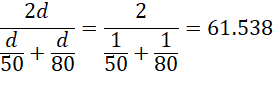
This is equivalent to the harmonic mean of 50 and 80, as calculated in Excel by the formula =HARMEAN(G7:G8) in cell G13 of Figure 2.

Examples Workbook

Click here to download the Excel workbook with the examples described on this webpage.

References

Wikipedia (2012) Mean
https://en.wikipedia.org/wiki/Mean

Microsoft (2021) HARMEAN function
https://support.microsoft.com/en-us/office/harmean-function-5efd9184-fab5-42f9-b1d3-57883a1d3bc6