Outliers from Normally-distributed Data
As explained in Identifying Outliers and Missing Data, for normally distributed data, we can identify an outlier as a data element outside the interval μ ± k ⋅ σ where k = 2.5, although k = 3.0 is also used. This is based on the fact that if the data is normally distributed (see Normal Distribution), then only 1.24% (about 1 out of 80) of the data elements would be outside this interval when k = 2.5, or 0.27% when k = 3.0.
Approach using IQR
The above approach is reasonable when the data are normally distributed. Otherwise, a non-parametric approach is preferred. In Box Plots with Outliers, we show how to identify outliers as data elements that are outside of the interval Median ± c ⋅ IQR where c = 1.5 (called Tukey’s fences) or 2.2.
Note that for normally distributed data, IQR ≈ 1.34898σ (see Property 4 of Measures of Variability) and Median = μ. Here 1.34898 = 2*NORM.S.INV(.75). Thus, k = 2.5 for the normal distribution becomes c = 2.5/1.34898 = 2.0235 ≈ 2 for this non-parametric version, and k = 3.0 for the normal distribution becomes c = 3.0/1.34898 = 2.239 ≈ 2.2. The other commonly used multiplier of c = 1.5 corresponds to a multiplier of k = 1.5*1.34898 = 2.0235 for the normal distribution, which seems quite low.
Approach using MAD
Another approach is to use the interval Median ± c ⋅ MAD where MAD is the median absolute deviation.
We first note that for normally distributed data, μ = Median and σ ≈ 1.4826 ⋅ MAD. Here, 1.4826 = 1/NORM.S.INV(.75). See Relationship between STD and MAD. Thus, for a normal distribution, the μ ± k ⋅ σ interval becomes Median ± 1.4826k ⋅ MAD. Thus, k = 2.5 for the normal distribution becomes c = 2.5 ⋅ 1.4826 = 3.7065 for this non-parametric version, and k = 3.0 for the normal distribution becomes c = 3.0 ⋅ 1.4826 = 4.4478.
Also see the Outliers using Median and MAD section of Identifying Outliers and Missing Data.
Example for Normally Distributed Data
Example 1: Determine the outliers for the data in column A of Figure 1.

Figure 1 – Outliers for normally distributed data
E.g. cells C11, D11 and F11 contain the formula =MEDIAN(A1:A19), =MAD(A1:A19) and =C11-D11*E11.
Since the data is normally distributed, all three approaches will yield similar results (except for the IQR approach with c = 1.5). E.g. based on the first approach with k = 2.5, there are no outliers since none of the data elements are outside the interval (-21.0624, 261.0624).
Example for Symmetric Data
Example 2: Determine the outliers for the data in column A of Figure 2.
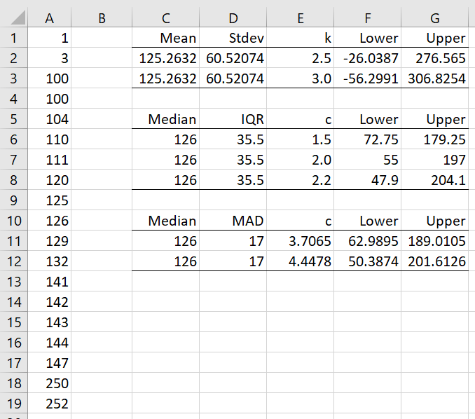
Figure 2 – Outliers for symmetrically distributed data
Since the data are symmetrically distributed but not normally distributed, we can use the IQR or MAD approach. The result is that 1, 3, 250, and 252 are potential outliers.
Extended Non-parametric Approaches
With data that is heavily skewed, we can benefit from using a Double MAD approach instead of the MAD approach described above. Click here for more details.
For some data sets (e.g. data coming from a bimodal distribution), we may find that using the Harrell-Davis median is a better approach than using the ordinary median when calculating the MAD or Double MAD. Click here for more details.
Links
Examples Workbook
Click here to download the Excel workbook with the examples described on this webpage.
References
Wikipedia (2021) Median absolute deviation
https://en.wikipedia.org/wiki/Median_absolute_deviation
Wikipedia (2021) Interquartile range
https://en.wikipedia.org/wiki/Interquartile_range
Akinshin, A. (2020) DoubleMAD outlier detector based on the Harrell-Davis quantile estimator
https://aakinshin.net/posts/harrell-davis-double-mad-outlier-detector/#Rosenmai2013