M-estimators

Basic Concepts

Certain measures of central tendency are more robust to outliers than others (e.g. the median is more robust than the mean). We now look at a class of statistics, the M-estimators, that serve as candidates for robust measures of central tendency. In particular, we consider two such estimators:  Tukey’s biweight estimator and Huber’s estimator.

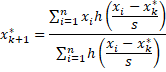
First, we note that since we want to reduce the weight of outliers we should consider weighted averages where more weight is assigned to data elements in the middle and less to the extreme values. For a data set x₁, …, x_n, such a weighted average takes the form

Note that the mean can be defined in this way where the weights are all assigned the value of 1. The trimmed mean can also be defined this way where w_i = 0 for the first and last p% of the i and w_i = 1 for the rest.

Tukey’s biweight

For Tukey’s biweight estimator, we choose weights such that

where

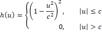
for the constant c = 4.685 and for s = MAD(x₁, x2, …, x_n). Note that x* is defined based on weights w_i that are in turn based on x*. This means that we need to calculate the weights and x* iteratively as follows:

We can test for convergence when for example

for some small positive value ε.

Example

Example 1: Calculate Tukey’s biweight estimator for the data in range A4:A23 of Figure 1.

The figure shows the calculation of the biweight estimator in Excel using 20 iterations (iterations 4 through 17 are not displayed), resulting in a value of 48.11807 (cell AU3). Actually, this level of precision was reached after only 13 iterations.

Figure 1 – Iterative calculation of Tukey’s biweight estimate

 The iteration is initialized by using the mean as the initial estimate of the biweight estimator (cell G3) via the formula =AVERAGE(A4:A23). The initial u values are shown in column F. E.g. u₁ = -2.54242 (cell F4) is calculated using the formula =($A4-G$3)/$D$6, where cell D6 contains the Real Statistics formula =MAD(A4:A23). Column G contains the initial weights. E.g. w₁ = .497738 (cell G4) is calculated using the formula

=IF(ABS(F4)<=$D$8,(1-F4^2/$D$8^2)^2,0)

where cell D8 contains c = 4.685.

We next calculate a new estimate for the biweight of 47.67484 (cell I3) using the formula

=SUMPRODUCT(G4:G23,$A$4:$A$23)/SUM(G4:G23)

We continue in this way getting better and better estimates (in cells K3, M3, etc.) for the biweight.

Huber’s estimator

Huber’s estimator is defined similarly using the formula

generally based on the value c = 1.339.

Worksheet Functions

Real Statistics Functions: The following functions are provided in the Real Statistics Resource Pack.

BIWEIGHT(R1, iter, prec, c, pure) = Tukey’s biweight estimate for the data in R1 based on the given cutoff c (default 4.685).

HUBER(R1, iter, c, prec) = Huber’s estimate for the data in R1 based on the given cutoff c (default 1.339).

iter = the number of iterations (default 50) and prec = the level of precision (default 0.00000001).

If the biweight estimate is undefined for the given value of c then when pure = FALSE (default) the value of c is increased until a valid biweight value is found, and when pure = TRUE then an error value is returned.

Unlike the biweight, the Huber function is always defined except when MAD(R1) = 0. In this case, when pure = TRUE, the function yields an error value, while if pure = FALSE then the function takes the value of MODE(R1). This is based on the fact that MAD(R1) = 0 only occurs when more than half the elements in R1 have the same value.

For Example 1, BIWEIGHT(A4:A23) = 48.11807 and HUBER(A4:A23) = 48.35514.

Examples Workbook

Click here to download the Excel workbook with the examples described on this webpage.

References

R-bloggers (2021) What is the Tukey loss function?
https://www.r-bloggers.com/2021/04/what-is-the-tukey-loss-function/

Wikipedia (2019) Huber loss
https://en.wikipedia.org/wiki/Huber_loss