The Real Statistics Resource Pack provides a variety of capabilities used for reformatting data. We explain a number of these capabilities on this webpage.
In addition to the capabilities described on this webpage, Real Statistics also provides the following reformatting worksheet functions:
- Sorting and duplicate removal functions QSORT, SortUnique, ExtractUnique, and NODUPES, plus the dynamic array functions SortsUnique, ExtractsUnique (see Sorting and Removing Duplicates).
- DELBLANK and DELNonNum, plus the dynamic array function DELROWS (see Dealing with Missing Data)
- SHUFFLE and RANDOMIZE, plus their dynamic array function versions SHUFFLES and RANDOMIZES. (see Sampling using Real Statistics Capabilities)
Worksheet Functions
Real Statistics Functions: The following array functions contained in the Real Statistics Resource Pack can be used to reformat data or to change the shape of an array or the order of elements in an array.
The following two functions are used to fill the highlighted cell range with the data from an array or cell range R1.
RESHAPE(R1, filler) – fills the highlighted range with the data in array or range R1 (in column order)
REVERSE(R1, filler) – fills the highlighted range with the data in array or range R1 in reverse order (by columns).
The string filler is used as a filler in case the output range has more cells than R1. This second argument is optional and defaults to the error value #N/A.
Other versions of RESHAPE and REVERSE
There is also another version of the RESHAPE and REVERSE array functions.
RESHAPE(R1, filler, nrows, ncols): outputs an nrows × ncols array with the data in array R1
REVERSE(R1, filler, nrows, ncols): outputs an nrows × ncols array with the data in array R1 in reverse order
This version of the two functions should only be used when called from within another function. E.g. suppose that you have a column array of numeric data in the range A1:A9, you could calculate the determinant of a 3 × 3 version of this data by using the array formula =MDETERM(RESHAPE(A1:A9,,3,3)).
Dynamic Array Functions
The Real Statistics Resource Pack also provides versions of these functions that are especially useful with versions of Excel that support dynamic arrays:
RESHAPES(R1, nrows, ncols, bycol): returns an nrows × ncols array with the elements from R1. If the nrows (ncols) argument is missing or 0, then nrows (ncols) is set to the smallest value such that all the elements in R1 are output. When nrows and ncols are both missing or 0, then a column array with all the elements in R1 is returned. If bycol = TRUE (default), then elements are returned in column order; otherwise, they are in row order. If R1 doesn’t contain a sufficient number of elements, then #N/A is used as a filler.
REVERSES(R1): outputs an array of the same size and shape as R1 with the data in range R1 in reverse order.
DELCOL(R1, ncol): returns an array just like the R1 array, but with the ncol-th column removed.
DELROW(R1, nrow): returns an array just like the R1 array, but with the nrow-th row removed.
Example 1
Reformat the data in range B5:D8 of Figure 1, as illustrated in the rest of the figure.
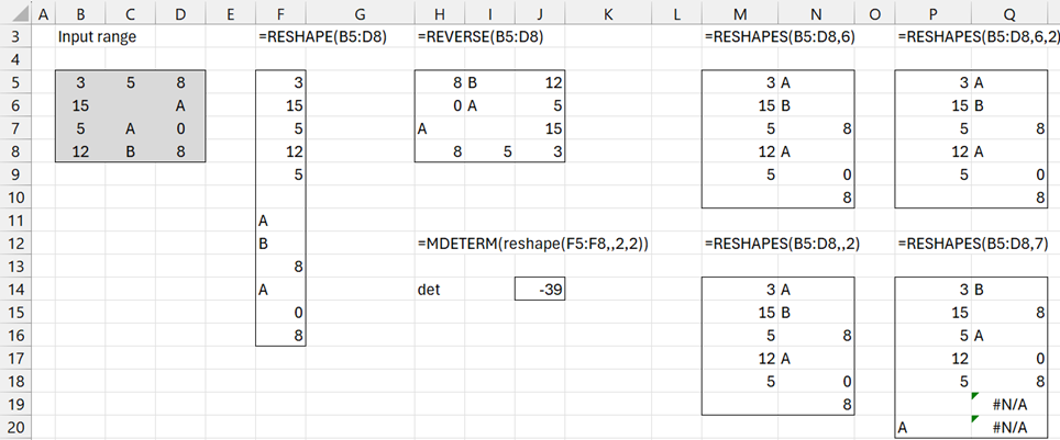
Figure 1 – Reshaping and reverse examples
Each example in the figure displays the use of the specified array formula in the range within the indicated rectangular border. E.g. the range F5:F16 contains the array formula =RESHAPE(B5:B8).
For versions of Excel that support dynamic arrays, the RESHAPES formulas can be entered in the upper-left cell in the indicated rectangle, and the entire rectangular region will be filled in with the output from that formula.
Other Worksheet Functions
The Real Statistics Resource Pack also supports the following array functions:
DELErr(R1): outputs an array of the same size and shape as R1 consisting of all the elements in R1 where any element with an error value is replaced by a blank (i.e. an empty cell).
MCONST(s, nrows, ncols): outputs an nrows × ncols array filled with the value s
SEQ(nrows, ncols, start, incr): outputs an nrows × ncols array containing the sequence of values start, start+incr, start+2*incr, start+3*incr… (in row order)
Here, start and incr default to 1. If nrows and/or ncols are omitted, then the dimensions of the highlighted range are used.
For example, the array formula =SEQ(2,3,5,4) outputs an array with 2 rows and 3 columns; the first row contains the values 5, 9, 13, and the second row contains the values 17, 21, 25. The output would be the same if you placed the array formula =SEQ(,,5,4) in range A1:C2.
MERGE(R1, R2): outputs an m × n1+n2 array which contains the values in the m2 × n2 cell array or range R2 adjoined to the right of the m1 × n1 cell array or range R1, where m = max(m1, m2) and any missing values are filled with blanks (or empty cells)
SUBMATRIX(R1, row1, col1, nrows, ncols): outputs an nrows × ncols subarray of the m × n array or cell range R1 starting at the cell in the row1th row and col1th column of R1.
Here, row1 and col1 default to 1. nrows defaults to m – row1 + 1, and ncols defaults to n – col1 + 1.
Example 2
Reformat the data in ranges B5:B7 and D5:E6 of Figure 2, as illustrated in the rest of the figure.
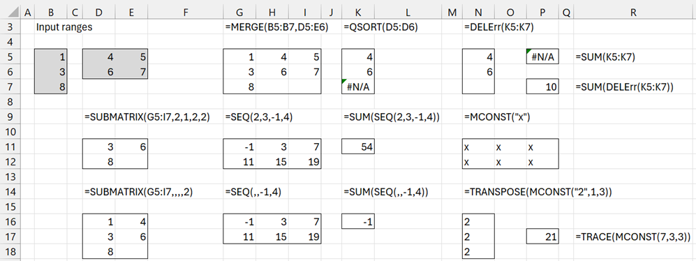
Figure 2 – More reformatting examples
Two Column Sequencing Worksheet Functions
The Real Statistics Resource Pack supports the following array functions:
SEQ2X(x1, xcount, y1, ycount, xincr, yincr): creates two sequences x1, x2, …, xm and y1, y2, …, yn, with m = xcount and n = ycount, and outputs an mn × 2 array with all possible pairs of values from these two sequences. Here, each element in the x sequence is separated from its predecessor by xincr (default 1), and each element in the y sequence is separated from its predecessor by yincr (default 1).
SEQ2S(x0, xm, y0, yn, xincr, yincr): creates two sequences x0, x1, …, xm and y0, y1, …, yn, and outputs a (m+1)(n+1) × 2 array with all possible pairs of values from these two sequences. Here, each element in the x sequence is separated from its predecessor by xincr (default 1), and each element in the y sequence is separated from its predecessor by yincr (default 1).
Figure 3 shows an example of the use of these functions.
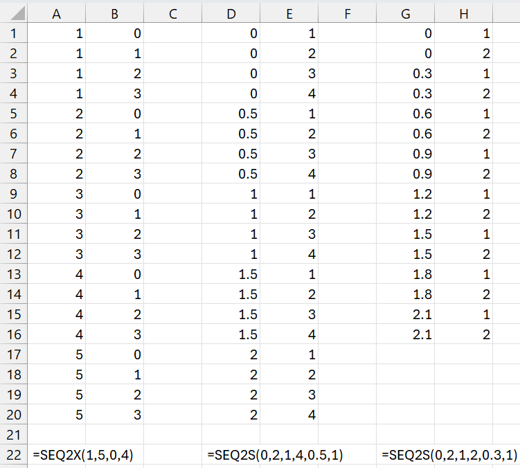
Figure 3 – SEQ2S and SEQX examples
Summary Tables
Real Statistics Functions: The Real Statistics Resource Pack contains the following array function that creates a summary table.
COMPACT(R1, head): returns an m × n array which is a summary table for the data in the h × k array R1. The first k-1 columns of the output consist of the unique values in the first k-1 values of R1. The remaining columns consist of the counts of rows in R1 that match the non-negative integer in the kth column of R1.
If the minimum value in the kth column of R1 is mn and the maximum value is mx, then the output contains an additional mx-mn+1 columns.
If head = TRUE (default FALSE) then the first row of R1 is assumed to contain column headings, in which case the elements in the first k-1 columns of the first row of R1 are retained as headings in the output and the headings for the remaining columns of the output are mn, mn+1, …, mx. If mx-mn > 24, then an error is generated.
Note that MLogitSummary(R1, head) and OLogitSummary(R1, head) are equivalent to COMPACT(R1, head). See Multinomial Regression Support and Ordinal Regression Support.
Example 3
Reformat the data in range A1:C16 of Figure 4 using the COMPACT worksheet function.
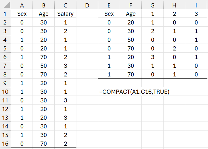
Figure 4 – COMPACT example
The array formula =COMPACT(A2,C16) produces the output shown in range E2:I8 of Figure 4.
Note that if you change the value in cell C16 to -1, then the output will contain two additional columns corresponding to headings of -1 and 0. All the entries for the column corresponding to 0 will be 0.
Binary version
The Real Statistics Resource Pack also provides a binary-choice version of COMPACT, defined as follows.
BCOMPACT(R1, head): returns an m × (k+1) array which is a summary table for the data in the h × k array R1 whose kth column can only contain the values 0 or 1. The first k-1 columns of the output consist of the unique values in the first k-1 values of R1. The kth column consists of the counts of the matching rows from R1 that contain 1 in the kth column, and the k+1th column consists of the counts of the matching rows from R1 that contain 0 in the kth column.
If head = TRUE (default FALSE) then the first row of R1 is assumed to contain column headings, in which case the elements in the first k-1 columns of the first row of R1 are retained as headings in the output, and the kth and k+1th columns of the first row contain the values “Success” and “Failure”.
Note that LogitSummary(R1, head) is identical to BCOMPACT(R1, head). See Logistic Regression Support.
Example 4
Reformat the data in range A1:C16 of Figure 5 using the BCOMPACT worksheet function.
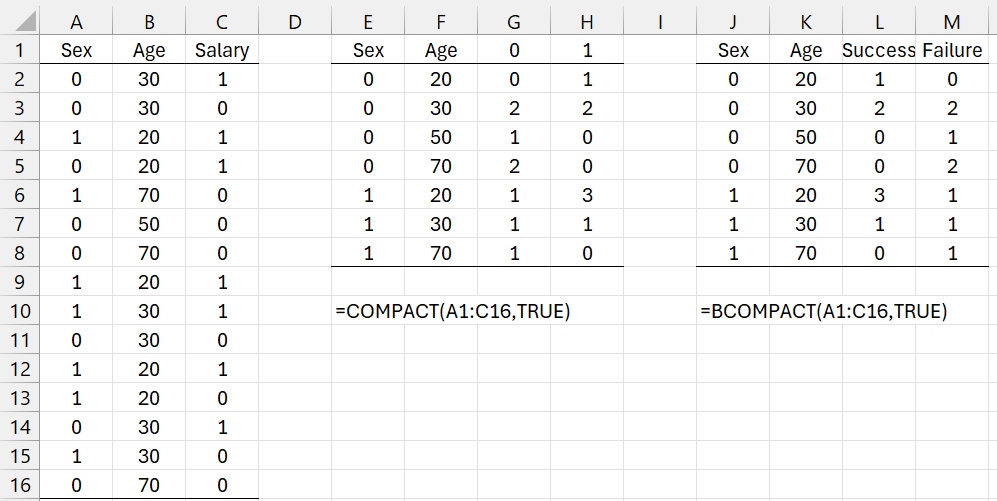
Figure 5 – BCOMPACT example
Data Analysis Tool
Real Statistics Data Analysis Tool: The Real Statistics Resource Pack contains the Reformatting a Data Range data analysis tool. This tool provides a variety of reformatting capabilities (including those provided by RESHAPES, REVERSES, and DELErr).
Example 5: Copy the data from range B5:D8 in Figure 1 into a 6 × 2 range by using the Reformatting a Data Range data analysis tool.
Press Ctrl-m, choose the Reformatting Data Range option (from the Desc tab if using the multipage user interface). A dialog box will appear as shown in Figure 6. Fill in the dialog box as indicated and click on the OK button. The output will appear in range M14:N19, as shown in Figure 1.
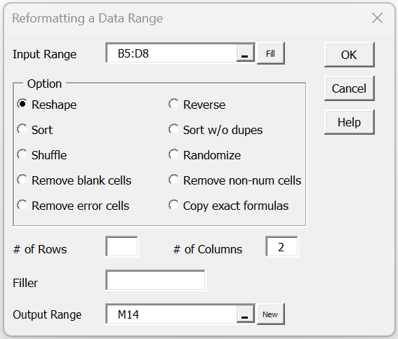
Figure 6 – Dialog box for Reformatting a Data Range
You don’t need to fill in the # of Rows field since the data analysis tool will automatically set its value to 6 (since 4 × 3 = 12 = 6 × 2).
Examples Workbook
Click here to download the Excel workbook with the SEQ2S and SEQ2X examples described on this webpage.
Click here to download the Excel workbook with the other examples described on this webpage.
Lists
↑ Data conversion and reformatting
References
Microsoft (2024) SEQUENCE function
https://support.microsoft.com/en-us/office/sequence-function-57467a98-57e0-4817-9f14-2eb78519ca90
Microsoft Support (2022) TOCOL function
https://support.microsoft.com/en-gb/office/tocol-function-22839d9b-0b55-4fc1-b4e6-2761f8f122ed
Hi!
So I came across your wonderful stat toolpak and I am eager to put it to good use. I have one question, I have noticed for analyzing, their is only one option which puts labels sorted as columns, however due to using my data in other programs for graphing and such, all of my data is organized as groups in rows. I was wondering if there is an easy way to use your tool pack without reformatting all of my data. I have about 6 sheets, each with 3-5 groups and 3 time-points. Thank you in advance!
Annette
Annette,
I can’t think of a way without reformatting your data. This can be done by using Excel’s TRANSPOSE function or by copying and pasting using the Transpose option.
Charles
After opening the sample files and updating to link to Real Stats there are many values which are now #NUM or #NAME and when looking at the formula it is changed to include path to real stats as in:
=’C:\Users\xx\AppData\Roaming\Microsoft\AddIns\RealStats.xlam’!COUNTU(A5:C8)
If I remove the path part I get message that there is some error in formula. How can I fix these. The above example came from Table Reformat 1 and except for original values all values in table are #NAME. Suggestions? Thank you
Kathleen,
When you update the link, the path name should go away. This is standard Excel.
You can get rid of the path name to get the formula =COUNTU(A5:C8).
See the following webpage for details: https://real-statistics.com/free-download/examples-installation/
Charles