Basic Concept
Recently, Microsoft has introduced a new type of array formula, available only with Excel 2021 and Excel 365. This type of array does not require that you highlight the output range and press Ctrl-Shift-Enter as described in Array Formulas and Functions.
To use a dynamic array formula with spillover, you enter the desired array formula in the top, left-most cell of the output range and simply press Enter. The output then automatically fills the rest of the range (this is the spillover). If you want to modify the formula, you only need to edit the cell that contains the formula. In fact, you cannot manually modify any of the other cells in the output range.
Examples
Example 1: Repeat Example 2 of Array Formulas and Functions using a dynamic array with spillover.
This time, you insert the formula =TRANSPOSE(A3:B8) in cell D3 and press Enter, as shown in Figure 1. The result is identical to that shown in Figure 2 of Array Formulas and Functions. Note that the formula is the same as that used in Example 2 of Array Formulas and Functions. The only difference is that you don’t need to specify the output range in advance; Excel figures this out for you.
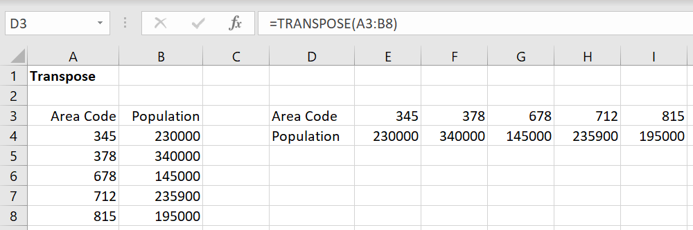
Figure 1 – Dynamic array formula
Note that the legacy formula {=TRANSPOSE(A3:B8)} displayed in the formula bar of Figure 2 of Array Formulas and Functions is enclosed in curly brackets {}. The dynamic array formula, however, is not enclosed in these brackets.
Spill Error
When using a dynamic array, no values or formulas can appear in the cells in the output range. Otherwise, a #SPILL! error value will appear.
For example, referring to Figure 1, if you insert any value, including 378, in cell F3, then cell D3 will change to the value #SPILL! Also, all the other cells in the range D3:I4 will be erased. In fact, if range D3:I4 is blank except that cell F3 contains some value or formula, then when you enter the array formula =TRANSPOSE(A3:B8) in cell D3 and press Enter, the error value #SPILL! will be displayed in cell D3 instead of the output shown in Figure 1.
The @ Operator
While you can’t use dynamic array formulas except in Excel 365, you can still use legacy array formulas in Excel 365, although you would be advised to use dynamic array formulas instead. Legacy array formulas (aka CSE array formulas for Ctrl-Shift-Enter) created in other versions of Excel will sometimes be preceded by an @ symbol. E.g. you may see =@TRANSPOSE(A3:B8) when using Excel 365.
Spilled Range Operator
Observation: Excel 365 also supplies a spilled range operator #. This operator can be used with a spilled range, i.e. a cell range that has been spilled over; e.g. the range D3:I4 in Figure 2.6.3. To specify this range in another formula, it is sufficient to use D3#. Therefore, if you want to insert the formula =D3:I4 in range D6:I7, it is sufficient to insert the formula =D3# in cell D6. Similarly, you could use a formula such as =SUM(D3#) instead of =SUM(D3:I4).
Note that you cannot use the formula =A3# in place of =A3:B8 since A3:B8 is not a spilled range.
Links
Examples Workbook
Click here to download the Excel workbook with the examples described on this webpage.
Reference
Microsoft (2020) Dynamic array formulas and spilled array behavior
https://support.microsoft.com/en-us/office/dynamic-array-formulas-and-spilled-array-behavior-205c6b06-03ba-4151-89a1-87a7eb36e531