Sorting and Filtering

Sorting

Excel provides a number of basic capabilities for sorting and filtering data in a worksheet. These capabilities are accessible from the Data ribbon.

Example 1: Sort the data in the range A3:D10 of Figure 1 by income

Figure 1 – Data to be sorted

Highlight the range A3:D12 and select Data > Sort & Filter|Sort. When the dialog box shown in Figure 2 appears, choose Income for the Sort by field and make sure that the My data has headers field is checked.

Figure 2 – Sort dialog box

Once you click on the OK button the data in range A3:D12 will be overwritten with the data in sorted order as shown in Figure 3.

Figure 3 – Data sorted by Income

Multiple Sorts

Now suppose that in the case of ties we wanted the entries to be sorted in alphabetic order by the person’s name. Notice that three people have an income of 35,000 and two have an income of 45,000. In neither case are the entries in alphabetic order by name. To perform a multilevel sort you need to press Add Level button in Figure 2. The dialog box will change to give you the opportunity to supply two sort keys. Fill in the entries as shown in Figure 4.

Figure 4 – Multiple level sort

This time the data will be sorted as shown in Figure 5.

Figure 5 – Data sorted by Income/name

Removing Rows with Missing Data

If you want to remove any rows from a range with an empty cell or a cell with non-numeric data, you can sort the range first. All the rows with an empty cell or cell with missing data will be moved to the end of the list where they can easily be removed. This is a way of removing rows of data with missing elements.

Removing Duplicates

Example 2: Remove any duplicates from the Income column of Figure 1.

Highlight the range D3:D10 and select Data > Data Tools|Remove Duplicates. The result is shown in Figure 6.

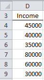
Figure 6 – Data without duplicates

Filtering

Example 3: Extract from the data in Figure 1 all the people who have income between 35,000 and 45,000 inclusive.

Highlight the range A3:D12 and select Data > Sort & Filter|Filter. The data will change as shown in Figure 7.

Figure 7 – Data after Filter is chosen

Click on the downward arrow in cell D3 and then select Number Filters on the dialog box that appears and then Greater Than Or Equal To… When the dialog box shown in Figure 8 appears, fill in the fields as shown and press the OK button.

Figure 8 – Filter dialog box

The result is shown in Figure 9.

Figure 9 – Filtered data

Examples Workbook

Click here to download the Excel workbook with the examples described on this webpage.

Reference

Pernsley, T. (2021) Sorting and filtering data with Excel. Learn Excel Now
https://www.learnexcelnow.com/sorting-and-filtering-data-with-excel/

References

University of Michigan (2025) Filtering and sorting data. Using Microsoft Excel
No longer available online
Microsoft (2026) How to sort and filter data (quick reference guide)
https://cdn-dynmedia-1.microsoft.com/is/content/microsoftcorp/microsoft/mcaps/documents/fy26/QRG-Sort-and-filter-data.pdf
“will not occur at the end of the list” -> “will be moved to the end of the list”
Konrad,
Thanks once again for finding this error. I have now made the change that you have suggested. I really appreciate your help in making the website more accurate and easy to understand.