Excel Charts

Excel provides fairly extensive capabilities for creating graphs, what Excel calls charts. You can access Excel’s charting capabilities by selecting Insert > Charts. We will describe how to create bar and line charts here. Elsewhere on the website, we describe how to create scatter charts. Other types of charts are created in a similar manner. Once a chart is created three new ribbons are accessible, namely Design, Layout, and Format. These are used to refine the chart created.

Bar charts

To create a bar chart execute the following steps:

1. Enter the data that you are charting into a worksheet.
2. Highlight the data range and select Insert > Charts|Column. A list of bar chart types is displayed. As usual, you can place the mouse pointer over the picture of any chart type to get a brief description of that chart type. E.g. the first type is a 2-dimensional side-by-side bar chart while the second choice is a 2-dimensional stacked bar chart.
3. Use the Design, Layout, and Format ribbons to refine the chart. At any time you can click on the chart to get access to these ribbons.

We now demonstrate how to create a bar chart via the following example.

Example

Example 1 – Create a bar chart for the data in Figure 1.

The first step is to enter the data into the worksheet. We next highlight the range A4:D10, i.e. the data (excluding the totals) including the row and column headings, and select Insert > Charts|Column.

Figure 1 – Bar Chart in Excel

The resulting chart is shown in Figure 1, although initially, the chart does not contain a chart title or axes titles. To add a chart title click on the chart, select Layout > Labels|Chart Title and then choose Above Chart and enter the title Marketing Campaign Results. You can add the title of the horizontal axis in a similar manner by selecting Layout > Labels|Axis Titles > Primary Horizontal Axis Title > Title Below Axis and entering the word City. Finally, you can add the title of the vertical axis by selecting Layout > Labels|Axis Titles > Primary Vertical Axis Title > Rotated Title.

Modifications

To get the results displayed in Figure 1 we also needed to move the chart within the worksheet by left-clicking on the chart and dragging it to the desired location. We can then resize the chart, making it a little smaller (or bigger), by clicking on one of the corners of the chart and dragging the corner to change the dimensions. To ensure that the aspect ratio (i.e. the ratio of the length to the width) doesn’t change it is important to hold the Shift key down while dragging the corner.

If instead of a chart of sales by city, you want a chart of sales by brand, you can click on the chart and select Design > Data|Switch Row/Column. You can also change the type of chart by clicking on the chart, selecting Design > Type|Change Chart Type, and then choosing the chart type that you want (e.g. a stacked bar chart instead of a side-by-side bar chart).

Line charts

The process for creating a line chart is similar to that of a bar chart. The main difference is that you need to select Insert > Charts|Line.

Example 2 – Create a line chart for the average income of a sample of people in their thirties by age based on the data in Figure 2.

Figure 2 – Line Chart (initial view)

To create the chart we highlight the range B3:B13 and select Insert > Charts|Line. The result is displayed in Figure 2. We next describe a series of modifications that we want to make to the chart.

The legend labeled Income is not particularly useful, and so we eliminate it by clicking on the chart and selecting Layout > Labels|Legend> None. We next change the chart title by simply highlighting the title (Income) and changing it to a more informative title such as Average Income by Age. We also insert the horizontal and vertical axes titles as we did for the bar chart in Example 1.

Note that the horizontal axis defaults to the time series 1 to 10 (since there are 10 data items). To change this to 31 to 40, we click on the chart and select Design > Select Data to display the dialog box shown in Figure 3.

Figure 3 – Edit axes labels dialog box

Now click on the Edit button for the Horizontal (Category) Axis Labels (on the right side of the dialog box). We are prompted for the axis label data range and enter A4:A13 (or simply highlight this range on the worksheet) and then press the OK button. We next press the OK button on the dialog box shown in Figure 3 to accept the change.

Modifications

Since no data element corresponds to income below 20,000 it might be better to have the vertical axis start with 20,000 instead of 0. We accomplish this by clicking on the vertical axis labels (0 to 40000) and selecting Layout > Current Selection|Format Selection Selection (alternatively, right-click on the vertical axis labels and choose the Format Axis… option). This opens the Format Axis dialog box. Select Axis Options and then change the radio button for Minimum from Auto to Fixed and enter 20000.

We also decide to change the formatting of the labels to use comma separators for thousands. This is accomplished by selecting the Number tab (which is also on the Format Axis dialog box), choosing the Number category, and then clicking the Use 1000 Separator (,) checkbox and entering 0 for the Decimal Places.

The result of all these modifications is shown in Figure 4.

Figure 4 – Line Chart (revised view)

Observation: You can also create charts with more than one line. Click here for more details.

Scatter charts

A scatter chart is simply a chart of a series of pairs of data elements, where the first data element corresponds to the x-axis and the second to the y-axis.

Example 3: Create a scatter chart of the (x, y) pairs shown in range A3:C9 of Figure 5. Here the pairs represent the revenues (y values) and operating costs (x values) in millions of dollars for each of the six divisions of a retail business.

Highlight the range B4:C9 and select Insert > Charts|Scatter and then modify the titles as we have done in previous examples to produce the chart shown in 5. Note that if the data rows were scrambled, we would get the same chart.

Figure 5 – Scatter Chart

If you want to add labels to each point in the chart with the appropriate district name, click on the chart. This brings up the three icons shown on the top right of the chart in Figure 5. Click on the + icon and then click to the right of the Data Labels chart element option.

On the menu that appears, select the More Options … choice. This brings up a menu as shown on the right side of Figure 6. Uncheck the Y Value option and check the Value from Cell option. In the dialog box that appears, enter the range A4:A9 (containing the district names) and press the OK button. The chart will now contain the district name labels as shown on the left side of Figure 6.

Figure 6 – Scatter Chart with labels

Step charts

Excel doesn’t provide a step chart capability, but we can create one by using the scatter chart capability shown above.

Example 4: Create a step chart for the data in Figure 7.

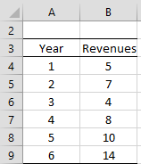
Figure 7 – Step chart data

The key is to re-enter the data found in A3:B9 of Figure 7 by duplicating the entries as shown in range J3:K14 of Figure 8. You can then highlight range J3:K14 (or J4:K14) and select Insert > Charts|Scatter, using the Scatter with Straight Lines and Markers option. After the usual modifications to the titles, you obtain the step chart shown in Figure 8.

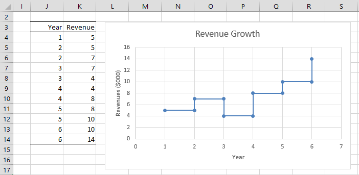
Figure 8 – Step Chart

Examples Workbook

Click here to download the Excel workbook with the examples described on this webpage.

References

Microsoft (2021) Create a chart from start to finish
https://support.microsoft.com/en-us/office/create-a-chart-from-start-to-finish-0baf399e-dd61-4e18-8a73-b3fd5d5680c2

Peltier, J. (2018) Step charts in Excel
https://peltiertech.com/step-charts-in-excel/