Excel has recently introduced a number of new dynamic array functions that can be used to reformat arrays. These worksheet functions are currently only available to Excel 365 users.
TOCOL and TOROW
TOCOL(R1, ignore, bycol): returns a column array with the elements in R1
TOROW(R1, ignore, bycol): returns a row array with the elements in R1
If ignore = 0 (default), then retain all the elements in R1; if ignore = 1 then ignore blanks; if ignore = 2 then ignore error values; if ignore = 3 then ignore blanks and error values
If bycol = TRUE then the output is in column order; otherwise (default), it is in row order.
Some examples are given in Figure 1.
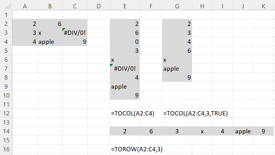
Figure 1 – TOROW and TOCOL examples
WRAPCOLS and WRAPROWS
WRAPCOLS(R1, size, filler): returns a two-dimensional array by column with size-many rows containing the elements in row or column array R1
WRAPROWS(R1, size, filler): returns a two-dimensional array by row with size-many columns containing the elements in row or column array R1
If there aren’t sufficient data elements in R1 then the remaining elements in the output are padded with filler (default #N/A).
Actually, if size is greater than or equal to the number of elements in R1 then R1 is returned (with no padding).
Some examples are provided in Figure 2.
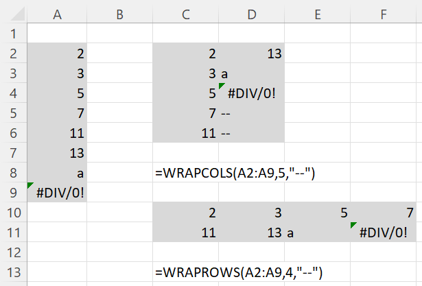
Figure 2 – WRAPROWS and WRAPCOLS examples
Note that you obtain the exact same output if you place the formula =WRAPCOLS(TRANSPOSE(A2:A9),5,”–“) in C2 and =WRAPROWS(TRANSPOSE(A2:A9),4) in cell C10.
CHOOSECOLS and CHOOSEROWS
CHOOSECOLS(R1, col1, col2, …): returns an array with the specified columns from R1
CHOOSEROWS(R1, row1, row2, …): returns an array with the specified rows from R1
Some examples are provided in Figure 3.
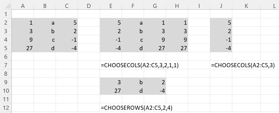
Figure 3 – CHOOSEROWS and CHOOSECOLS examples
EXPAND
EXPAND(R1, nrows, ncols, filler): expands R1 to nrows rows and ncols columns.
This function returns an nrows × ncols array whose upper left subarray is R1. All the expanded elements are padded with filler (default #N/A).
If nrows is omitted then no rows are appended. Similarly, if ncols is omitted then no columns are appended.
If the number of rows in R1 is less than nrows or the number of columns in R1 is less than ncols, an error results.
Some examples are displayed in Figure 4.
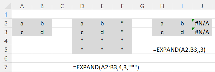
Figure 4 – EXPAND examples
DROP and TAKE
DROP(R1, nrows, ncols): eliminates rows and/or columns from R1.
If nrows > 0 then the first nrows rows are eliminated. Similarly, if ncols > 0 then the first ncols columns are eliminated.
If nrows is omitted (or zero) then no rows are eliminated. Similarly, if ncols is omitted (or zero) then no columns are eliminated.
If nrows < 0 then the last –nrows rows are eliminated. Similarly, if ncols < 0 then the last –ncols columns are eliminated.
If the number of rows in R1 is less than nrows or the number of columns in R1 is less than ncols, an error results.
Some examples are displayed in Figure 5.
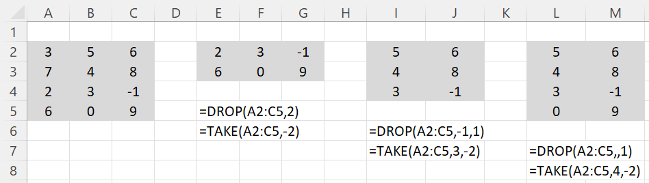
Figure 5 – DROP and TAKE examples
TAKE(R1, nrows, ncols): extracts rows and/or columns from R1.
If nrows > 0 then the first nrows rows are extracted. Similarly, if ncols > 0 then the first ncols columns are extracted
If nrows is omitted then only columns are extracted. Similarly, if ncols is omitted then only rows are extracted.
If nrows < 0 then the last –nrows rows are extracted. Similarly, if ncols < 0 then the last –ncols columns are extracted.
We see from Figure 5, that any subarray that can be specified by a DROP formula can also be specified by an equivalent TAKE formula and vice versa.
Note that the array formula =TAKE(TAKE(A2:C4,,2),,-1) produces the middle column (whose values are those in B2:B4) of the array on the left side of Figure 5.
HSTACK and VSTACK
HSTACK(R1, R2, …): stacks R1, R2, … horizontally (appends R2 to the right of R1, etc.); the resulting array has m rows where m = the maximum # of rows in R1, R2, …; if necessary #N/A is used as padding
VSTACK(R1, R2, …): stacks R1, R2, … vertically (appends R2 below R1, etc.) .); the resulting array has n columns where n = the maximum # of columns in R1, R2, …; if necessary #N/A is used as padding
If you want to use something else as padding, then you can do this via a formula of the form
=IFERROR(HSTACK(R1, R2, …), filler)
and similarly for VSTACK. Some examples are displayed in Figure 6.
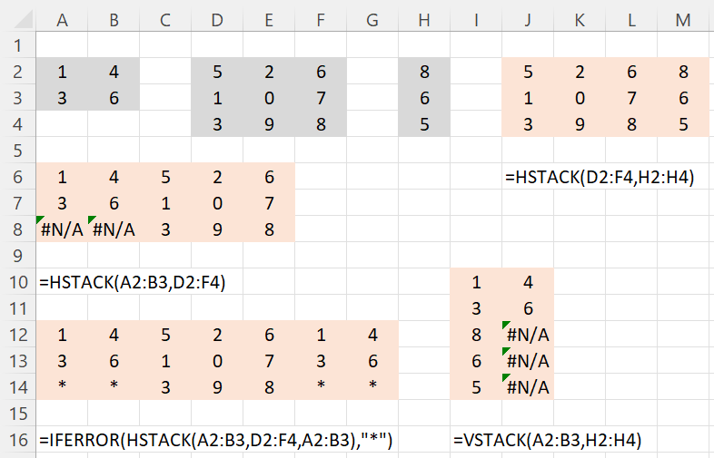
Figure 6 – HSTACK and VSTACK examples
Examples Workbook
Click here to download the Excel workbook with the examples described on this webpage.
References
McDaid, J. (2022) Announcing new text and array functions. Microsoft Tech Community
https://techcommunity.microsoft.com/t5/excel-blog/announcing-new-text-and-array-functions/ba-p/3186066
Microsoft Support (2022) TOCOL function
https://support.microsoft.com/en-gb/office/tocol-function-22839d9b-0b55-4fc1-b4e6-2761f8f122ed