Sorting and Removing Duplicates

Excel provides standard capabilities for sorting and eliminating duplicates. These can be accessed by Data > Sort & Filter|Sort and Data > Data Tools|Remove Duplicates. See Sorting and Filtering for more details.

Sorting functions have only been provided in the most recent releases of Excel (see Sorting and Filtering Functions). For earlier versions of Excel, sorting using Excel functions is possible using a little ingenuity, as described in Sorting using Excel Formulas.

The Real Statistics Resource Pack provides a number of sorting functions available for all releases of Excel. We describe these capabilities on this webpage. These capabilities can also be accessed via Real Statistics data analysis tools.

Worksheet Functions

Real Statistics Functions: The following array functions contained in the Real Statistics Resource Pack can be helpful in sorting data and removing duplicates.

QSORT(R1, ascend, nrows, ncols) – returns an nrows ⨯ ncols array with the data in range R1 in sorted order (arranged by columns) ); ascend is an optional parameter (default = TRUE); if ascend is TRUE then the sort is in ascending order and if ascend is FALSE (or 0) the sort is in descending order

SortUnique(R1, filler) – fills the highlighted range with the data in range R1 in ascending sorted order eliminating any duplicates (arranged by columns); the highlighted range should only have one column

ExtractUnique(R1, filler) – fills the highlighted range with the data in range R1 in the order found in R1 (arranged by columns) eliminating any duplicates; the highlighted range should only have one column

NODUPES(R1, filler, b) – fills the highlighted range with the data in range R1 eliminating any duplicates (arranged by columns); if b = TRUE then the data in R1 is sorted first, and if b = FALSE then it is assumed that range R1 is already in sorted order.

The string filler is used as a filler in case the output range has more cells than R1. This second argument is optional and defaults to the error value #N/A.

For QSORT, if nrows = 0 or is omitted then the output array is the highlighted range on the active worksheet. If nrows < 0 then the output is an array of the same size and shape as R1; in both these cases, ncols  is not used and can be omitted; otherwise ncols defaults to 1.

For the above functions, data in a range is assumed to be ordered first by column and then by row. E.g. for the range A1:B2, the presumed order is A1, A2, B1, B2.

Examples

The following two figures provide examples of the use of the above worksheet functions. Each example displays the use of an array formula in the range within the indicated rectangular border.

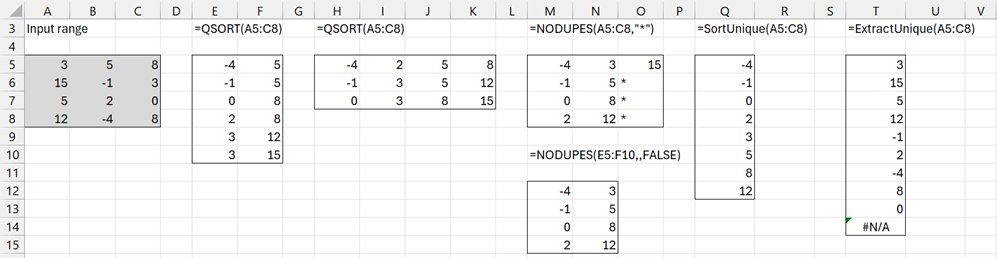
Figure 1 – Numeric examples

E.g. the range E5:F10 contains the array formula =QSORT(A5:C8). Note that range M12:N15 is not large enough to hold all 9 unique values and so 15 is omitted.

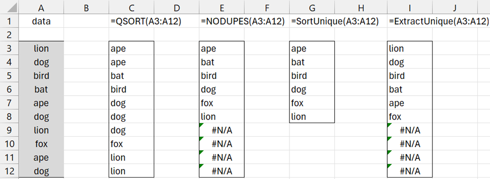
Figure 2 – Alphanumeric examples

Dynamic Real Statistics Functions

There are also the following functions that are useful with dynamic arrays:

SortsUnique(R1) – outputs a column array with the data in range R1 in ascending sorted order eliminating any duplicates

ExtractsUnique(R1) – outputs a column array with the data in range R1 in the order found in R1 eliminating any duplicates

Example

Figure 3 provides examples of the use of the above two functions, plus QSORT when the row and column lengths are specified. For these examples, Excel 365 uses can enter each formula in the upper left corner of the highlighted rectangle and press the Enter key.

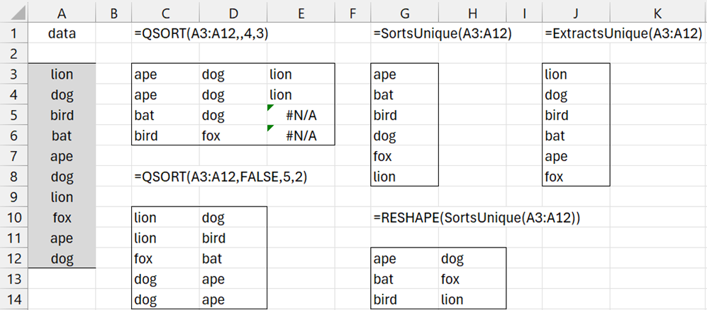
Figure 3 – Dynamic array formulas

Data Analysis Tool

Real Statistics Data Analysis Tool: The Real Statistics Resource Pack contains the Reformatting a Data Range data analysis tool. This tool provides a variety of reformatting capabilities (including those provided by QSORT and SortsUnique).

See Example 5 from Reformatting Capabilities for more details.

Count Worksheet Functions

Real Statistics Functions: The Real Statistics Resource Pack also provides the following non-array worksheet functions related to the  ExtractsUnique function.

COUNTU(R1) = count of the number of unique numeric elements in R1

COUNTAU(R1) = count of the number of unique non-blank elements in R1

R1 is an array or cell range that doesn’t contain any error values.

For example, referring to Figure 1, the formula =COUNTU(B5:D8) returns the value 9. Similarly, referring to Figure 2, the formula =COUNTAU(A3:B12) returns the value 6.

Examples Workbook

Click here to download the Excel workbook with the examples described on this webpage.

References

Mellor, L. (2020) Sort and filter using dynamic array functions in Microsoft Excel
https://www.laramellortraining.co.uk/how-to-sort-and-filter-using-dynamic-array-functions-in-microsoft-excel

Stack Overflow (2021) Sortby function combined with Unique combined with filter functions
https://stackoverflow.com/questions/68246608/sortby-function-combined-with-unique-and-filter-functions-how-to-use-it-correcl