Introduction
As in Sampling Distributions, we can consider the distribution of r over repeated samples of x and y. The following property is analogous to the Central Limit Theorem, but for r instead of x̄. This time we require that x and y have a joint bivariate normal distribution or that the samples are sufficiently large. You can think of a bivariate normal distribution as the three-dimensional version of the normal distribution, in which any vertical slice through the surface of the graph of the distribution results in an ordinary bell curve.
Key Property
The sampling distribution of r is only symmetric when ρ = 0 (i.e. when x and y are independent). If ρ ≠ 0, then the sampling distribution is asymmetric and so the following property does not apply, and other methods of inference must be used.
Property 1: Suppose ρ = 0. If x and y have a bivariate normal distribution or if the sample size n is sufficiently large, then r has a normal distribution with mean 0, and t = r/sr ~ T(n – 2) where
![]()
Here the numerator r of the random variable t is the estimate of ρ = 0 and sr is the standard error of r.
If we solve the equation in Property 1 for r, we get
![]()
As we will see, this fact will prove to be relevant for Property 2 of Correlation in Relationship to t-Test.
Property 1 can be used to test the hypothesis that population random variables x and y are independent i.e. ρ = 0 (assuming bivariate normality).
Example (two-tailed)
Example 1: A study is designed to check the relationship between smoking and longevity. A sample of 15 men 50 years and older was taken and the average number of cigarettes smoked per day and the age at death was recorded, as summarized in the table in Figure 1. Can we conclude from the sample that longevity is independent of smoking?
![]()
Figure 1 – Data for Example 1
The scatter diagram for this data is as follows. We have also included the linear trend line that seems to best match the data. We will study this further in Linear Regression.

Figure 2 – Scatter diagram for Example 1
Next, we calculate the correlation coefficient of the sample using the CORREL function:
r = CORREL(R1, R2) = -.713
From the scatter diagram and the value of the correlation coefficient r, it is clear that the population correlation is likely to be negative. The absolute value of the correlation coefficient looks high, but is it high enough? To determine this, we establish the following null hypothesis:
H0: ρ = 0
Recall that ρ = 0 would mean that the two population variables are independent. We use t = r/sr as the test statistic where sr is as in Property 1. Based on the null hypothesis, ρ = 0, we can apply Property 1, provided x and y have a bivariate normal distribution. It is difficult to check for bivariate normality, but we can at least check to make sure that each variable is approximately normal via QQ plots.

Figure 3 – Testing for normality
Both samples appear to be normal, and so by Property 1, we know that t has approximately a t distribution with n – 2 = 13 degrees of freedom. We now calculate
![]()
 Test Results
Finally, we perform either one of the following tests:
p-value = T.DIST.2T(ABS(-3.67), 13, 2) = .00282 < .05 = α (two-tail)
tcrit = T.INV.2T(.05, 13) = 2.16 < 3.67 = |tobs|
And so we reject the null hypothesis and conclude there is a non-zero correlation between smoking and longevity. In fact, it appears from the data that increased levels of smoking reduce longevity.
The various calculations are shown in Figure 4.
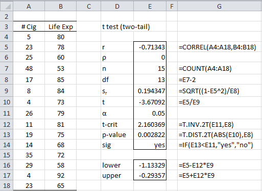
Figure 4 – Hypothesis testing of the correlation coefficient
We also see that the 95% confidence interval for the population correlation coefficient ρ is (-1.13, -.294). Note that 0 is not in this interval, confirming once again that there is a non-zero correlation between smoking and longevity.
Example (one-tailed)
Example 2: The US Census Bureau collects statistics comparing the various 50 states. The table in Figure 5 shows the poverty rate (% of the population below the poverty level) and infant mortality rate per 1,000 live births) by state. Based on this data, can we conclude the poverty and infant mortality rates by state are correlated?

Figure 5 – Data for Example 2
The scatter diagram for this data is shown in Figure 6.
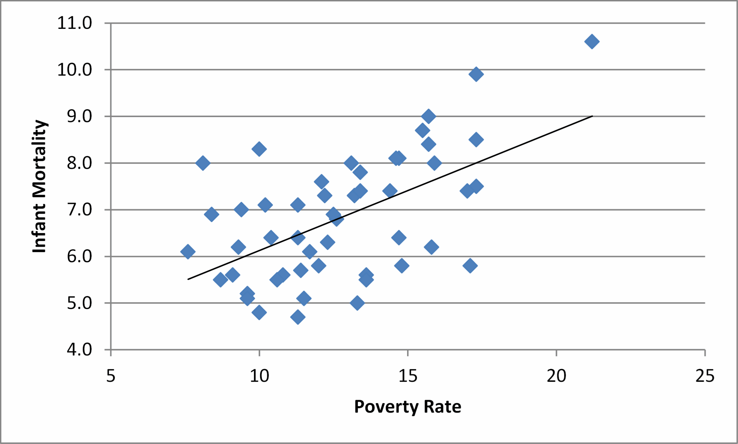
Figure 6 – Scatter diagram for Example 2
The correlation coefficient of the sample is given by
r = CORREL(B4:B53, C4:C53) = .564
Since the population correlation was expected to be non-negative, the following one-tail null hypothesis was used:
H0: ρ ≤ 0
Based on the null hypothesis we will assume that ρ = 0 (best case), and so as in Example 1
![]()
![]()
Finally, we perform either one of the following tests:
p-value = T.DIST.RT(4.737, 48) = 9.8E-06 < .05 = α (one-tail)
tcrit = T.INV(.95, 48) = 1.677 < 4.737 = tobs
In either case, we reject the null hypothesis and conclude there is a non-zero correlation between poverty and infant mortality.
Since we were confident that the correlation coefficient wasn’t negative, we chose to perform a one-tail test. It turns out that even if we had chosen a two-tailed test (i.e. H0: ρ = 0), we would have still rejected the null hypothesis.
Worksheet Functions
Real Statistics Functions: The following functions are provided in the Real Statistics Resource Pack.
CorrTTest(r, size, tails) = the p-value of the one-sample test of the correlation coefficient using Property 1 where r is the observed correlation coefficient based on a sample of the stated size. If tails = 2 (default) a two-tailed test is employed, while if tails = 1 a one-tailed test is employed.
CorrTLower(r, size, alpha) = the lower bound of the 1 – alpha confidence interval of the population correlation coefficient based on a sample correlation coefficient r coming from a sample of the stated size.
CorrTUpper(r, size, alpha) = the upper bound of the 1 – alpha confidence interval of the population correlation coefficient based on a sample correlation coefficient r coming from a sample of the stated size.
CorrelTTest(r, size, alpha, lab, tails): array function which outputs t-stat, p-value, and lower and upper bounds of the 1 – alpha confidence interval, where r and size are as described above. If lab = TRUE then output takes the form of a 4 × 2 range with the first column consisting of labels, while if lab = FALSE (default) then output takes the form of a 4 × 1 range without labels.
CorrelTTest(R1, R2, alpha, lab, tails) = CorrelTTest(r, size, alpha, lab, tails) where r = CORREL(R1, R2) and size = the common sample size, i.e. the number of pairs from R1 and R2 for which both pair members contain numeric data; i.e. COUNTPair(R1, R2, FALSE).
If alpha is omitted it defaults to .05. If tails = 2 (default) a two-tailed test is employed, while if tails = 1 a one-tailed test is employed.
Observation: For Example 1, we observe that CorrTTest(-.713, 15) = .00282, CorrTLower(-.713, 15, .05) = -1.13 and CorrTUpper(-.713, 15, .05) = -.294.
Also =CorrelTTest(A4:A18,B4:B18,E11,TRUE) produces the output shown in Figure 7.
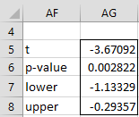
Figure 7 – CorrelTTest output
Critical Values
As observed earlier
![]()
We can use this fact to create the critical values for the t-test described above, namely

Real Statistics Function: The following function is also provided in the Real Statistics Resource Pack.
PCRIT(n, α, tails) = the critical value of the t-test for Pearson’s correlation for samples of size n, for the given significance level α (default .05), and tails = 1 (one tail) or 2 (two tails, default).
A table of such critical values can be found in Pearson’s Correlation Table.
Examples Workbook
Click here to download the Excel workbook with the examples described on this webpage.
References
Howell, D. C. (2010) Statistical methods for psychology (7th ed.). Wadsworth, Cengage Learning.
https://labs.la.utexas.edu/gilden/files/2016/05/Statistics-Text.pdf
OpenStax (2023) Testing the significance of the correlation coefficient
https://stats.libretexts.org/Bookshelves/Introductory_Statistics/Introductory_Statistics_(OpenStax)/12%3A_Linear_Regression_and_Correlation/12.05%3A_Testing_the_Significance_of_the_Correlation_Coefficient
how is this different from T.Test from excel
The goal of this test is to determine whether the correlation coefficient is significantly different from zero.
The T.Test is used to determine whether there is a significant difference between the means of two samples.
It turns out that these two tests are equivalent as described at https://www.real-statistics.com/correlation/dichotomous-variables-t-test/
Charles
hello there …
if i have two variables, each one with 1460 entry and i want to calculate correlation between them , what is the appropriate test, i used Pearson correlation, and the result is not good, r=0.25 and p almost zero, how i could judge if two variables are related to each other or not
What is a 1460 entry?
Charles
thanks
I am calculating percentage bias of simulated and reference time series, can I use same function with bias instead of r to do the test?
Monzer,
I don’t completely understand your question.
Charles
Hi Charles, thanks for this post and for the whole website which is excellent. I was wondering whether it is possible to use your t formula to test whether a correlation is significantly different from a value other than 0, say .70, by simply putting (r – .70) at the numerator? From what I know about the one-sample t-test, that makes sense. But as it is sometimes suggested to use a Fischer’s Z-transformation to test the significance of correlations, I was wondering whether my rationale was practically correct with the t-test. Thanks in advance. Best regards
Hello Nico,
I am pleased that you like the website.
The following webpage describes correlation tests. The t-test is only value for 0. For other values, you need to use Fisher’s transformation.
https://real-statistics.com/correlation/one-sample-hypothesis-testing-correlation/
Charles
Hi, Charles,
I am running Pearson’s and Spearman’s correlation tests on about 600 pairs of air and water temperature observations. The outputs from both of these tests gave me a “p-value” of “0.” Either I made a mistake or I need to increase the number of decimal places – can you help me? I have pasted the Pearson’s output below.
Thanks much. Love the product!
Correlation Coefficients
Pearson 0.485848391
Spearman 0.477471802
Kendall 0.333101533
Pearson’s coeff (t test)
Alpha 0.05
Tails 2
corr 0.485848391
std err 0.032108776
t 15.13132727
p-value 0
lower 0.422813388
upper 0.548883395
Hello Leo,
If you email me an Excel file with your data, I will try to figure out what is happening.
Charles
how can i report the results of the correlation that utilized t test ?
Hello Hasan,
Are you referring to the APA way of reporting results?
Charles
Would please let me know the reference for theorem 1
Theorem 1: “Suppose ρ = 0. If x and y have a bivariate normal distribution or if the sample size n is sufficiently large, then r has a normal distribution with mean 0, and t = r/sr ~ T(n – 2) where…”
Hello Hamid,
You will find this in many textbooks. E.g. the Howell textbook referenced in the Bibliography.
Charles
i want to post the numerical value or data for representative of graph
please how i post my data for interpret the figure and table .
Hello,
I don’t understand what you mean by “post your data”. Are you asking how to format your data? For this test, you can format your data in many ways, but especially as two columns of equal size.
Charles
A correlation coefficient(r) of 0.2 is derived from a random sample of 625 pairs of observations. Is this value of r significant? Also carry out a %9 5confidence interval to the population correlation coefficient.
Hello Denis,
If by significant you mean that the correlation coefficient is significantly different from zero, then this webpage describes how you can test for significance and determine confidence intervals.
Charles
Hey Charles,
Sorry for haranguing on Example 2 again! The p-value I get from my spreadsheet is 9.8E-06, not 9.8E-08. Additionally, TINV(.05, 48) returns the two-tailed inverse for me. I have to enter T.INV(.95,48) to return the indicated value of 1.677.
Can you confirm if my assumptions are correct? Much appreciated!
David,
You are correct on both accounts. Please keep haranguing me. I really appreciate knowing when the website has a mistake in it. Your haranguing has been very helpful. Thanks.
Charles
Hey David,
It seems that the t-test done in Example 2 is the right-tailed t-test. If the correlation coefficient is negative, would you perform the left tailed t-test? When would it be proper to perform a standard two-tailed test?
Thanks.