An alternative to using Fisher’s transformation or the exact test for one-sample correlation testing is to use resampling techniques, bootstrapping and randomization, as described in Resampling Procedures and Resampling Data Analysis Tool.
Example
Example 1: Repeat Example 5 of One-sample Correlation Hypothesis Testing using bootstrapping. In particular, find the 95% confidence interval for the correlation coefficient for the samples shown in range A4:B11 of Figure 1.
The correlation coefficient for the sample data is calculated by CORREL(A5:A11,B5;B11) = .97292 (cell B13). Range A15:B18 shows the results of the analysis using the Fisher transformation. We now explain the rest of Figure 1.
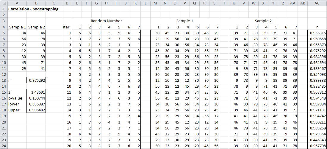
Figure 1 – Bootstrapping of the correlation coefficient
We start by generating 2,000 random sample pairs based on pairs from the original sample and then calculate the correlation coefficient of each of these pairs. Since the original sample consists of 7 pairs, each bootstrap sample should consist of 7 pairs. Since we want to make sure that pairs from the original sample stay together (e.g. if 34 is included in a bootstrap sample then it should be paired with 46 from Sample 2 and not 78 or some other value in Sample 2), we randomly generate 7 numbers between 1 and 7 with replacement and use these values as indices to the two original samples.
Figure 1 shows the first 20 of the 2,000 random bootstrap samples. The first pair of bootstrap samples is shown in ranges M5:S5 and U5:AA5 of Figure 1. The 7 random numbers used to generate this pair is shown in range E5:K5. Each of the cells in this range contains the formula =RANDBETWEEN(1, 7). Cell M5 contains the formula =INDEX($A$5:$A$11,E5) and cell U5 contains the formula =INDEX($B$5:$B$11,E5).
In fact once the formulas in cells E5, M5 and U5 are inserted, all the others can be generated by (1) highlighting range E5:K2004 and pressing Ctrl-R and then Ctrl-D, (2) highlighting range M5:S2004 and pressing Ctrl-R and then Ctrl-D and (3) highlighting range U5:AA2004 and pressing Ctrl-R and then Ctrl-D.
Calculating the correlation for each bootstrap pair
Next, we need to calculate the values of the correlation coefficient for each bootstrap sample pair. This can be done by inserting the formula =CORREL(M5:S5,U5:AA5) in cell AC5, highlighting the range AC5:AC2004 and pressing Ctrl-R and Ctrl-D. The result consists of 2,000 correlation coefficients in range AC5:AC2004. We can now create a frequency table and histogram of these values, as shown in Figure 2.
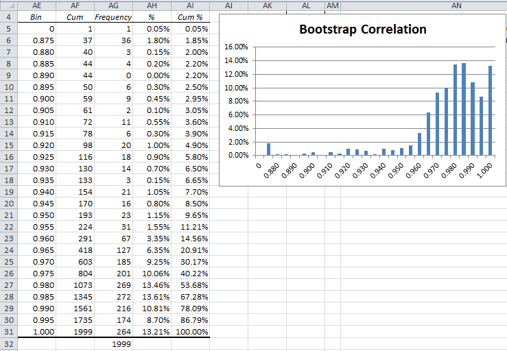
Figure 2 – Frequency table and histogram
We observe that the bootstrap correlations are not normally distributed. We also observe that the total number of samples (cell AG32) doesn’t come out to 2,000 as expected. This is because one of the pairs of bootstrapped samples has zero standard deviation (since all the sample values are the same) and so the correlation coefficient is undefined.
Estimating the confidence interval
Since there are 2,000 iterations and α = .05, the lower end of the confidence interval is the 2,000 · .025 = 50th smallest of the bootstrapped correlation coefficients, while the upper end of the confidence interval is the 50th largest of the bootstrapped correlation coefficients. The resulting confidence interval (.894, .999) can be calculated in Excel as shown in Figure 3.

Figure 3 – Confidence interval
Data Analysis Tool
Real Statistics Data Analysis Tool: We now show how to perform the above analysis using the Resampling data analysis tool.
Press Ctrl-m and double-click on the Resampling data analysis tool from the menu. Next fill in the dialog box that appears as shown in Figure 4 and click on the OK button.
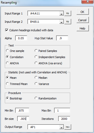
Figure 4 – Resampling dialog box
The output includes a frequency table and histogram similar to that shown in Figure 2, plus the output shown in Figure 5.

Figure 5 – Bootstrapping for correlation coefficient
The correlation coefficient of the original samples (A5:A11 and B5:B11 of Figure 1) is 0.975292 (cell AQ37). Since the hypothetical population correlation coefficient of .9 is less than .975292, the left-tailed p-value (.024 in cell AQ38) is the count of all bootstrapped correlation coefficients that are less than .9 divided by 2,000 (the total number of bootstrapped correlations generated).
Since .975292 – .9 = .075292, the right-tailed p-value (cell AQ39) is the count of all bootstrapped correlation coefficients that are larger than 0.975292 + .075292 = 1.050584 divided by 2,000. But since 1.050584 > 1, the right-tailed p-value is 0. The two-tailed p-value is the sum of the left and right tails, which is .024 + 0 = .024. Since this value is less than α, we conclude that the population correlation coefficient is significantly different from .9, which is different from the conclusion we reached using the Fisher transformation in Example 5 of One-sample Correlation Hypothesis Testing.
Figure 5 also shows the 95% confidence interval of (.901627, .998899) produced by the resampling data analysis tool. The mean of all the bootstrapped correlation coefficients is .972337 (cell AQ44) with standard deviation .039079 (cell AQ45).
Resampling Option
If the Resampling option is chosen instead of the Bootstrapping option, then the hypothesized population correlation coefficient is assumed to be zero and sampling is done without replacement. Each sample pair now consists of all the elements in sample 1 (range A5:A11) in their original order together with the elements in sample 2 (range B5:B11) in random order (equivalent to using the SHUFFLE function).
Examples Workbook
Click here to download the Excel workbook with the examples described on this webpage.
References
Howell, D. C. (2010) Statistical methods for psychology (7th ed.). Wadsworth, Cengage Learning.
https://labs.la.utexas.edu/gilden/files/2016/05/Statistics-Text.pdf
Efron, B. and Tibshirani, R. J. (1993) An introduction to the bootstrap. Springer
Howell, D. C. (2015) Bootstrapping correlations
https://www.uvm.edu/~statdhtx/StatPages/Randomization%20Tests/BootstCorr/bootstrapping_correlations.html
Hi Charles
I have just recently discovered the Real Statistics package, and am extremely grateful for your excellent work in putting it together, covering a wide spectrum of statistical techniques.
I wonder whether you would introduce the BCA confidence intervals (CI) as outlined in Chapter 14 of Efron and Tibshirani’s book on An Introduction to the Bootstrap, in a future update of the package. Looking at the histogram of the 1999 correlation coefficients from the bootstrap, it is seen that the distribution is very much skewed to the left. As a result, the bootstrap percentile CI is expected to have poor coverage rates. The theory suggests that one would get better coverage rates with BCA CIs than percentile CIs.
Best regards.
Siu-Ming
Hi Siu-Ming,
I’ll look into this.
Charles
Hi Charles
Thanks.
FYI, I used the data in your well-explained example and found that with the 95% percentile CIs, the coverage rate for r, amongst the 2000 bootstrap estimates, was 89.8% and for the 95% BCA CI, 97.7%.
Best regards.
Siu-Ming
Hi Siu-Ming,
Thanks for bringing this to my attention. I am reading Efron and Tibshirani’s book now.
Charles
Hi Charles
My apologies. The figures in the previous email are wrong – I have made an error in the Excel s/s. Also, it is not correct to assess coverage accuracy using the bootstrap estimates. The 1996 Statistical Science paper by DiCicio and Efron entitled Better Confidence Intervals lays out the proper way to do it.
Thanks.
Siu-Ming
Hello Siu-Ming,
Are you saying that the confidence intervals that you referred to in Efron and Tibshirani’s book are not as good as the approach in the DiCicio and Efron paper?
Charles
Hi Charles
You asked “Are you saying that the confidence intervals that you referred to in Efron and Tibshirani’s book are not as good as the approach in the DiCicio and Efron paper?”.
No, I did not mean to say that. The BCa method outlined in the book and the paper is the same and therefore equally good. For example, both sources recommend the use of the same functions of the Jackknife to estimate the acceleration for BCa confidence interval construction.
Jackknife is already included in your well-resourced package under the Cross Validation tab – LOOCV, hence the BCa method sits comfortably in any future expanded package.
I referred to the D&E paper because in its Table 2, it shows the coverage rate of the BCa Confidence Intervals (CIs) for the correlation coefficient under a bivariate normal distribution is spot on, giving evidence that the BCa methodology is a better method (second order accurate in theory) than the standard method (+/- 1.96 * SD) for CIs (first order accurate).
Of course, one does not know how good the BCa CIs if the underlying distribution is unknown but can take a leap of faith that it will do well, based on the results of Table 2.
Regards.
Siu-Ming
Thanks for the clarification.
I have now read chapter 14 and will try to figure out how best to add BCa CI support.
Charles
Hi again Dr. Charles;
I need your consultation;
I have 2 populations, 1st is a health providers at 2 hospitals (supervisory staff) with total sample size of (328 person) and the 2nd population is the in-patient at the same 2 hospitals with total sample size of (540 pts.). 2 surveys was used to collect the data, one survey for each population, the 1st one (with 68 questions) for the 1st population used to measure the level of using Six Sigma Methodology (DMAIC) at 2 hospitals, and 2nd one (with 36 questions) for the 2nd population that used to measure the level of patient’s satisfaction under light of using Six Sigma Methodology (DMAIC) at the same 2 hospitals. Both surveys has the same 5 dimensions (DMAIC) with same Likert Scale (5 scale), the data was collected at the same times. There are difference in questions no. between the 2 surveys, but there are (13) similar questions in every survey.
I need to find the effect or association (correlation) between the level of using Six Sigma Methodology (DMAIC) as (X variable) and the level of patient’s satisfaction under light of using Six Sigma Methodology (DMAIC) as (Y variable) using the data that collected as mentioned above. So I do the following:
1. Assuming that, level of pt. satisfaction is the Y variable, so I fixed every pt.’s case score (average mean for every dimension and total mean score), then we have 540 pts. with (6 scores for every one).
2. Also I assuming that, level of Using Six Sigma Methodology (DMAIC) is the X variable, then I measure the score for every health provider case (total of 328 person), so I have 6 scores for every one (average mean for every 5 dimensions and total mean score).
3. Using bootstrapping technique to generate random samples form the scores of health provider cases that every random sample contain (10) cases of them together which starting with a certain generated no. and calculate the scores, then return back the cases for the origin samples.
4. Repeat previous step (3) starting with a new generated no. to be sure not repeat the same generated random sample.
5. With step (3) and (4), using bootstrap, so we have (1000) random samples for each (540) pt. cases.
6. From the previous steps we will calculate the correlation between (X) and (Y).
My question is that: Is this procedure right or accurate to calculate the association between X and Y?, if Yes, which test can I used to perform it?, if No, How to do this right?.
best regards; Amer
See response to your most recent comment.
Charles
Thank you Charles! Worked perfectly–got the p value (by typing in “=CorrTTest(F8,24,2)” where F8 = the correlation, 24 = sample size, 2 = 2-tailed). I seem to be having difficulty using the “CNTRL-M” command on my MAC so I’ve been typing “=” to enter the formulae.
Thanks again,
Bill
Good to hear Bill. I believe that you use Comand-m in the Mac instead of Ctrl-m.
Charles
Thanks Charles! I’ll give this a shot and see how goes in the next day or 2. You’re a GEM and I really appreciate all your efforts on this. I’ve introduced my graduate students to your work and they, too, are very appreciative of your efforts. Will be back with feedback after I’m able to try out your Resampling tool.
Best, Bill
Hi Dr. Zaointz. Thank y0u very much for your efforts on this. I am a PhD-level researcher/Associate Professor who conducts lots of statistical analyses (using SPSS, JMP, recently experimenting with R, etc.) on my grant-funded research, and your excel tools (newly discovered) are extremely helpful.
I do have two question about the reliability analyses you’ve created in excel:
1) Once conducting the tests (e.g., correlations, Spearman-Brown correlations) and getting the r values, how can one get the p-value for the corresponding r-value? I’m creating reliability summary tables and would like to add the p-value next to the r values.
2) Using your “Split_Half” function (i.e., =SPLIT_HALF(B3:B26,C3:C26)) and copying your formula for the Spearman-Brown correction (=2*F4/(1+F4)) yield the same output. Does the Split_Half function automatically calculate the Spearman-Brown correction?
Thank you very much for your wonderful work on these tools and for your response to my inquiry!
Best, Bill
Hello Bill,
1) You can use the Correlation data analysis tool to calculate the p-values of the various supported correlation tests.
How to do this is described in the Correlation webpages. See Correlation.
See, especially Correlation Data Analysis Tool
2) Yes, the Split_Half function (and the equivalent in the Cronbach’s Alpha data analysis tool) do automatically calculate the Spearman-Brown correction.
Charles