Introduction
Suppose we conduct an ANOVA and reject the null hypothesis that all the sample means are equal. Since there are significant differences among the means, it would be useful to find out where the differences are. To accomplish this we perform extended versions of the two-sample comparison t-tests described in Two Sample t-Test with Equal Variances.
In fact, some bypass the omnibus ANOVA altogether and jump immediately to the comparison tests. Using this approach, as we will see, only the value of MSE from ANOVA is required for the analysis.
For example, suppose you want to investigate whether a college education improves earning power, considering the following five groups of students:
- High School Education
- College Education: Biology majors, Physics majors, English majors, History majors
You select 30 students from each group at random and find out their salaries 5 years after graduation. The omnibus ANOVA shows there are differences between the mean salaries of the four groups. You would now like to pinpoint where the differences lie. For example, you could ask the following questions:
- Do college-educated people earn more than those with just a high school education?
- Do science majors earn more than humanities majors?
- Is there a significant difference between the earnings of physics and biology majors?
Null hypotheses
The null hypothesis (two-tail) for each of these questions is as follows:
=


These tests are done employing something called contrasts.
Contrasts
Definition 1: Contrasts are simply weights ci such that
![]()
The idea is to turn a test such as the ones listed above into a weighted sum of means
![]()
using the appropriate values of the contrasts as weights. For example, for the first question listed above, we use the contrasts
![]()
and redefine the null hypothesis as
![]()
We then use a t-test as described in the following examples. Note that we could have used the following contrasts instead:
![]()
The results of the analysis will be the same. The important thing is that the sum of the contrasts adds up to 0 and that the contrasts reflect the problem being addressed.
For the second question, by using the contrasts
![]()
the null hypothesis once again can be expressed in the form:
The third question uses contrasts
Example
Example 1: Compare methods 1 and 2 from Example 3 of Basic Concepts for ANOVA.
We set the null hypothesis to be:
H0 : µ1 – µ2 = 0, i.e. neither method (Method 1 or 2) is significantly better
When the null hypothesis is true, this is the two-sample case investigated in Two Sample t-Test with Equal Variances where the population variances are unknown but equal. As before, we use the following t-test
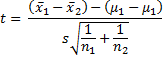
which has distribution T(n1 + n2 – 2).
But as we have seen, s2 = MSW and dfW = n1 + n2 – 2, and so when the null hypothesis is true,
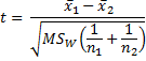
which has distribution T(dfW). For Example 1, we have the following results:

Figure 1 – Comparison test of Example 1
Since p-value = .02373 < .05 = α, we reject the null hypothesis and conclude that there is a significant difference between methods 1 and 2.
t-statistic for contrasts
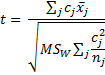
In fact, there is a generalization of this approach, namely the use of the statistic

where the cj are constants such that c1 + c2 + c3 + c4 = 0. As before t ~ T(dfW). Here the denominator is the standard error. We now summarize this result in the following property.
Property
Property 1: For contrasts cj, the statistic t has distribution T(dfW) where
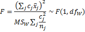
Since by Property 1 of F Distribution, t ~ T(df) is equivalent to t2 ~ F(1, df), it follows that Property 1 is equivalent to
Example 1 (continued): We can use Property 1 with c1 = 1, c2 = -1 and c3 = c4 = 0 as follows:

Figure 2 – Use of contrasts for Example 1
Here the standard error (in cell N14) is expressed by the formula =SQRT(I15*R11) and the t-stat (in cell O14) is expressed by the formula =S11/N14. As before p-value = .0237 < .05 = α.
Confidence Intervals
The t-test can also be used to create a confidence interval for a contrast, exactly as was done in Confidence Interval for ANOVA.
Example 2: Compare method 4 with the average of methods 1 and 2 from Example 3 of Basic Concepts of ANOVA.
We test the following null hypothesis
H0: µ1 = (µ2 + µ3) / 2
using Property 1 with c1 = 1, c2 = c4 = -.5 and c3 = 0.

Figure 3 – Use of contrasts for Example 2
Since p-value = .9689 > .05 = α, we can’t reject the null hypothesis, and so conclude there is no significant difference between method 4 and the average of methods 1 and 2.
One-tailed test
The above analysis employs a two-tail test. We could also have conducted a one-tail test using the null hypothesis H0: µ1 ≤ (µ2 + µ3) / 2. In that case, we would use the one-tail version of T.DIST in calculating the t-stat.
Orthogonal Contrasts
Contrasts are essentially vectors, and so we can speak of two contrasts being orthogonal. Per Definition 8 of Matrix Operations, assuming that the group sample sizes are equal (i.e. ni = nj for all i, j), contrasts (c1,…,ck) and (d1,…,dk) are orthogonal provided
![]()
Geometrically this means the contrasts are at right angles to each other in space.
Assuming there are k groups, if you have k – 1 contrasts C1, …, Ck-1 that are pairwise orthogonal, then any other contrast can be expressed as a linear combination of these contrasts. Thus you only ever need to look at k – 1 orthogonal contrasts. Since
![]() for any contrast C = (c1,…,ck), each of the Cj is orthogonal to the unit vector (1,…,1) and so k – 1 contrasts (and not k) are sufficient.
for any contrast C = (c1,…,ck), each of the Cj is orthogonal to the unit vector (1,…,1) and so k – 1 contrasts (and not k) are sufficient.
Note that if C1, …, Ck-1 are pairwise orthogonal, then SS between groups,
![]()
Also each
![]()
and so
![]()
Relationship to omnibus ANOVA
Thus any k – 1 pairwise orthogonal contrasts partition SSB.
Thus, if none of the t-tests for a set of k–1 pairwise orthogonal contrasts are significant, then the ANOVA F-test will also not be significant. Consequently, if the omnibus ANOVA F-test is significant, then at least one of k–1 pairwise orthogonal contrasts will be significant.
A non-significant F-test does not imply that all possible contrasts are non-significant. Also, a significant contrast doesn’t imply that the F-test will be significant.
In general, to reduce experiment-wise error you should make the minimum number of meaningful tests, preferring orthogonal contrasts to non-orthogonal contrasts. The key point is to make only meaningful tests.
Unbalanced samples
When the group sample sizes are not equal (i.e. unbalanced group samples), we need to modify the definition of orthogonal contrasts. In fact, contrasts (c1,…,ck) and (d1,…,dk) are orthogonal provided
![]()
The assumptions for contrasts are the same as those for ANOVA, namely
- Independent samples
- Within each group, participants are independent and randomly selected
- Each group has the same population variance
- Each group is drawn from a normal population
The same tests that are employed to test the assumptions of ANOVA (e.g. QQ plots, Levene’s test, etc.) can be used for contrasts. Similarly, the same corrections (e.g. transformations) can be used for contrasts. In addition, two other approaches can be used with contrasts, namely Welch’s correction when the variances are unequal or a rank test (e.g. Mann-Whitney U test or ANOVA on ranked data) when normality is violated. Keep in mind that ranks are only ordinal data, and so linear combinations (including averages) cannot be used, only comparisons of type µ1 = µ2. Also, any conclusions drawn from ANOVA on ranked data apply to the ranks and not the observed data.
Dealing with Experiment-wise error
As described in Experiment-wise Error Rate, in order to address the inflated experiment-wise error rate, either the Dunn/Sidák or Bonferroni correction factor can be used.
Dunn/Sidák correction was described in Experiment-wise Error Rate. To test k orthogonal contrasts in order to achieve an experiment-wise error rate of αexp, the error rate α of each contrast test must be such that 1 – (1 – α)k= αexp. Thus α = 1 – (1 – αexp)1/k. E.g. if k = 4 then to achieve an experiment-wise error rate of .05, α = 1 – ∜.95 = 0.012741.
Bonferroni correction simply divides the experimental-wise error rate by the number of orthogonal contrasts. E.g. for 4 orthogonal contrasts, to achieve an experiment-wise error rate of .05, simply set α = .05/4 = .0125. Note that the Bonferroni correction is a little more conservative than the Dunn/Sidák correction, since αexp/ k < 1 – (1 – αexp)1/k.
In the above calculations, we have assumed that the contrasts have equal values for α. This is not strictly necessary. E.g. in the example above, for the Bonferroni correction, we can use .01 for the first three contrasts and .02 for the fourth. The important thing is that the sum be .05 and that the split be determined prior to seeing the data.
If the contrasts are not orthogonal then the above correction factors are too conservative, i.e. they over-correct.
Example
Example 3: A drug is being tested for its effect on prolonging the life of people with cancer. Based on the data on the left side of Figure 3, determine whether there are significant differences in the 4 groups, and check (1) whether there is a difference in life expectancy between the people taking the drug and those taking a placebo, (2) whether there is a difference in the effectiveness of the drug between men and women and (3) whether there is a difference in life expectancy for people with this type of cancer for men versus women.

Figure 3 – Data and ANOVA output for Example 4
The ANOVA output in Figure 3 shows (p-value = .00728 < .05 = α) there is a significant difference between the 4 groups. We now address the other questions to try to pinpoint where the differences lie. First, we investigate whether the drug provides any significant advantage.

Figure 4 – Contrast test for effectiveness of drug in Example 3
Figure 4 shows the result with uncontrolled type I error and then the results using the Bonferroni and Dunn/Sidák corrections. The tests are all significant, i.e. there is a significant difference between the population means of those taking the drug from those in the control group taking the placebo.
We next test whether there is a difference in the effectiveness of the drug between men and women.

Figure 5 – Contrast test for men vs. women
Since p-value = .0547 > α in all the tests, we conclude there is no significant difference between the longevity of men versus women taking the drug.
The final test is to determine if men and women with this type of cancer have a different life expectancy (whether or not they take the drug).

Figure 6 – Contrast of life expectancy of men vs. women
The result is significant (p-value = .0421 < .05 = α) if we don’t control for type I error, but the result is not significant if we use the Bonferroni or Dunn/Sidák correction (p-value = .0421 > .0167 = α).
Worksheet Function
Real Statistics Function: The Real Statistics Resource Pack provides the following function:
DunnSidak(αexp, k) = α = 1 – (1 – αexp)1/k
Data Analysis Tool
Real Statistics Data Analysis Tool: The Real Statistics’ Single Factor Anova and Follow-up Tests data analysis tool provides support for performing contrast tests. The use of this tool is described in Example 4.
Example 4: Repeat the analysis from Example 2 using the Contrasts option of the Single Factor Anova and Follow-up Testssupplemental data analysis tool.
Enter Ctrl-m and select Single Factor Anova and Follow-up Tests from the menu. A dialog box will appear as in Figure 7.
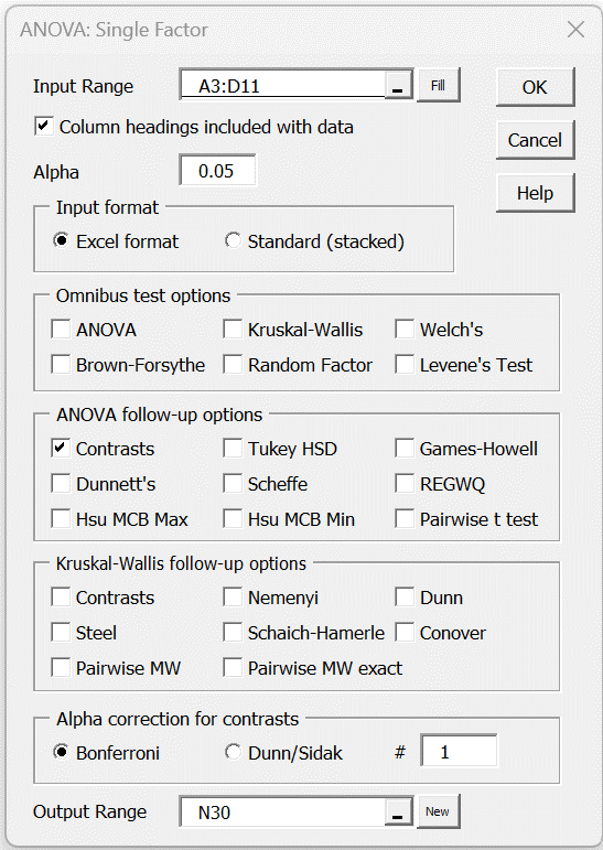
Figure 7 – Dialog box for Single Factor Anova and Follow-up Tests
Enter the sample range in Input Range, click on Column headings included with data, and check the Contrasts option. Select the type of alpha correction that you want, namely no experiment-wise correction, the Bonferroni correction, or the Dunn/Sidák correction (as explained in Experiment-wise Error Rate). In any case, you set the alpha value to be the experiment-wise value (defaulting as usual to .05).
Output
Note too that the contrast output that results from the tool will not contain any contrasts. You need to fill in the desired contrasts directly in the output (e.g. for Example 4 you need to fill in the range O32:O35 in Figure 7 with the contrasts you desire).
When you click on OK, the output from this tool is displayed (as in Figure 8). The fields relating to effect size are explained in Effect Size for ANOVA.

Figure 8 – Real Statistics Contrast data analysis
Caution
If your Windows settings for the decimal separator is comma (,) and the thousands separator is period (.) then you may get incorrect values for alpha when using the Bonferroni or Sidak/Dunn corrections.
To avoid this problem, you need to configure Real Statistics to use the correct settings, as described at Using Comma as the Decimal Symbol.
Examples Workbook
Click here to download the Excel workbook with the examples described on this webpage.
Reference
Howell, D. C. (2010) Statistical methods for psychology (7th ed.). Wadsworth, Cengage Learning.
https://labs.la.utexas.edu/gilden/files/2016/05/Statistics-Text.pdf
Wikipedia (2012) Bonferroni correction
https://en.wikipedia.org/wiki/Bonferroni_correction
Abdi, H. (2007) The Bonferonni and Šidák corrections for multiple comparisons
https://personal.utdallas.edu/~herve/Abdi-Bonferroni2007-pretty.pdf
Charles,
In Ex. 1, you have substituted the standard deviation with MSw and df of the t test with n1+n2-2. In this case, MSw should be the MS based on only Method 1 and Method 2, rather than all 4 methods, shouldn’t it?
Based on the Figure 1, it seems that you have used MSw based on all 4 methods and df of 25, which is from all 4 methods. However, we are comparing only Method 1 and Method 2 means. Therefore, the df should be 13 instead of 25.
I compared the results using the two sample equal variance t-test to the results using MSw using 4 methods and df of 25, they did not match. When I used MSw using only 2 methods (ie, Method 1 and Method 2) and df=13, the results match with the 2 sample equal variance t-test results.
Please advise.
Sun Kim,
It is not surprising that the results will be different. If you are only going to do one planned follow-up pairwise test (i.e. you know in advance of seeing the data which pairwise test you will do and you will only do one such test), then you should just perform the usual t test. In other cases, you should do one of the planned or unplanned post-hoc tests.
Charles
Hello Charles,
Can you please clarify the use of Bonferroni’s correction in the following ANOVA & planned comparisons scenario. I have a data set with 3 experimental groups and 3 dependent variables. I would like to perform 3 separate one-way ANOVAs. (I can’t perform MANOVA because Box’s M test shows inhomogeneity of covariance matrices). I assume that I should divide the required alpha for the main effect of each of the 3 ANOVAs by 3, and require p< 0.167, for each main effect, correct? Is this still the case if I also wish to perform (planned) paired comparisons (by Tukey's HSD test) on two of the 3 ANOVAs that showed significant main effects? Since there are 3 groups, each ANOVA will require 3 paired comparisons, for a total of 6 paired comparisons. Does this change the Bonferroni’s correction applied for the main effect of each ANOVA, , i.e. should I still require p < 0.05/ 3= 0.167 for the main effect of each ANOVA, or should I require p< 0.05/9 because a total of 9 tests will be performed, 3 for main effects and 6 for Planned comparisons? And for the paired comparisons on each ANOVA, should I use p < 0.05/3, or p < 0.05/6 because I am doing 6 paired comparisons, or p < 0.05/9 because I am doing a total of 9 tests (3 for main main effects and 6 for paired comparisons)?
Thanks very much.
Joel
Joel,
I believe that your reasoning is correct. If you plan to perform Tukey’s HSD for each of 3 ANOVAs, then you would use a corrected alpha of .05/3. If instead you planned to perform Tukey’s HSD on ANOVAs A and B and 3 paired comparisons on ANOVA C, then you would use .05/5 (one for A and B and 3 for C). Etc.
The ANOVAs themselves are typically not counted.
Charles
Charles,
Sorry but I am still confused about whether to apply the Bonferroni to both the ANOVAs & the paired comparisons or only to the paired comparisons. I think I need to frame my question more precisely so that I understand your reply.
Original plan was to perform 3 separate ANOVAs, one for each of the dependent variables A, B, and C, followed by paired comparisons on only the ANOVAs that showed main effects (Only A and B showed main effects, both at p<0.001. For C, p= 0.09). When you said “The ANOVAs themselves are typically not counted” did you mean that p<0.05 (I.e. no Bonferroni correction required) was appropriate for all 3 ANOVAs?
And for the paired comparisons, of which there were 6 (3 for A and 3 for B), what is the appropriate Bonferroni correction for these? Should I use p < 0.05/6, or 0.05/3? Doesn’t the Tukey HSD test have its own built-in correction when using the Real Statistics program?
Sorry to be so verbose but I was having trouble understanding your reply.
Thanks very much.
Hi Charles,
I would like to perform power and sample size calculations for a one-way ANOVA with three levels of the independent variable, A, B, & C. I know how to perform power and sample size calculations for one way ANOVA. Does Real Statistics support sample size and power calculations for planned comparisons using Tukey HSD following ANOVA)?
Thanks very much.
Joel
Joel,
Real Statistics does not yet support sample size and power for Tukey’s HSD. See
https://www.researchgate.net/deref/http%3A%2F%2Fdigitalcommons.wayne.edu%2Fcgi%2Fviewcontent.cgi%3Farticle%3D1291%26context%3Djmasm
Charles
I have 16 model permutations that I want to compare with my control group using ANOVA with contrasts and Tukey HSD follow-up and the Bonferroni alpha correction. Both follow up methods identify 4 model permutations that have significant results. I’d like to narrow the results even further by conducting another iteration of the ANOVA and followup tests to see if the 4 models results remain significant. What are the potential implications of running successive iterations of these tests?
Scott,
The situation you are describing is not completely clear to me. Are you saying that you have 17 “treatments” including a control group? By significant result, do you mean that 4 treatments are significantly different from the control group? It is not clear to me why you would perform both contrasts (presumably with a Bonferroni correction) and Tukey HSD.
Charles
Dear Charles,
I want to test differences between four groups of kids:
group A doesn’t practice any sport (control group)
groups B,C,D do practice different sports
so, by assuming one-way ANOVA results significant, I want to test if there are differences between control group and sports group (A vs B+C+D) and also between each pair of sports group (that is, B vs C, B vs D, C vs D).
These contrasts are not orthogonal because the test is unbalanced (different group sizes).
I think that the Real Statistics contrast analysis is the right approach to be used in my case, but which is the right correction factor I should use, in order to keep the experiment-wise error rate to alpha=0.05?
And conversely, if I wish to test all possible pairs of means, what could be the better approach, being the sample unbalanced?
Thank you very much for your help
Best Regards
Piero
Piero,
1. If you have 4 contrasts then the Bonferroni correction is .05/4 = .0125 (the Dunn/Sidák correction is similar).
2. If you want to test all possible pairs, then the Tukey-Kramer Test is probably the way to go (assuming homogeneity of variances). See
https://real-statistics.com/one-way-analysis-of-variance-anova/unplanned-comparisons/
Charles
Charles,
thank you very much. Just a clarification on point 1:
being the 4 contrasts not independent, does the Bonferroni/Dunn-Sidak corrections still apply with the same formulas as for orthogonal contrasts?
Piero
Piero,
You just use k = 4 since this is the number of tests used, irrespective of orthogonality.
If you have orthogonality, then the number of tests that you need will be limited.
Charles
Hello Charles,
I installed the program and ran a one-way ANOVA for some data with three groups. The ANOVA was significant, and now I would like to know which group is different. I’m trying to run some multiple comparison test, like Games-Howell, but it’s not working. I’m using the Excel in a Macbook, and actually, in my options when I open the program I do not have “Single Factor Anova and Follow-up Tests “, just “Analysis of Variance”. What can be happening? Thank you, Bárbara!
Bárbara,
Unfortunately, the Mac version uses an older release of the software and doesn’t have all the capabilities found in the Windows version.
Charles
Oh, ok! Thank you for your answer.
Bárbara!
Thanks Charles!
if its not too much to ask, could you send me an email that i could send a more exemplified question? just need to know i am doing the right thing. thanks for your response
Terry, just click on Contact Us on top menu to get my email address. Charles
could you kindly elaborate on how to to fill in the desired contrasts directly in the output. i am lost.
Terry,
E.g. you would fill in the contrasts in the range O7:O10 in Figure 2. Initially all the cells in this range are blank and you need to fill in contrast values that sum to 0 such that the positive values add up to 1 and the negative values add up to -1. E.g. 1, 0, -1. 0 or -.5, +.5, +.5, -.5.
Charles
Hi Charles,
When I try Dunn/Sidak correction and Bonferroni Correction, I get an error:
‘A run time error has occurred. The analysis tool will be aborted. Type Mismatch.’
If I do contrasts with no correction, then it’s fine. but not the other 2 options.
Declan
Declan,
Thanks for reminding me about this error. It is related to the fact that some users employ a period as the decimal point and other use a comma. I have now resolved this problem, and it should be fixed in the next release of the software, which will be available later this week.
Charles
Good day Charles 🙂
I often think that a t test with equal variances is more like an academic exercise. For example, nobody knows what the population mean or population standard deviation is, yet there are equations for it. If you don’t know it, use the sample standard deviation/mean etc. Based on this assumption, I’ve been applying the same logic to t tests- as it’s unlikely that the samples with have the same variances.
Interesting comment though that you made about the variance of one sample needs to be four times the variance of the other sample. Didn’t know that. Thanks. 🙂 In R, I think I’ve been doing the same thing VAR.EQUAL=FALSE. 🙂 But I will now have to be more careful.
Merry Christmas to you.
Declan
Declan,
Keep in mind that “variance of one sample needs to be at most four times the variance of the other sample” is a rule-of-thumb”. To be on the safe side you can always use the test with unequal variances. When the variances are equal or fairly equal the results will be almost the same as the t test with equal variances.
Charles
Thanks Charles 🙂
Hi,
Could please tell me, where we use t-test for equal variance or Unequal variance.
I am bit confused.
Thanks in Advance.
Rajeev,
When the variances of the two samples are relatively equal then the results of the two tests are approximately the same. It turns out that the t-test with equal variances gives a good result even when the variances are pretty unequal, but when the variance of one of the samples is quite different (approximately when the variance of one sample is more than four times the variance of the other sample), you should use the t-test with unequal variances instead of the t-test with equal variances.
Since the t-test with unequal variances can always be used (at least where the other assumptions for the t-test are satisfied), when in doubt just use this test.
Charles
Sir,
Could you please give me some guidance about how to do the planned contrast for the categorical dependent variable?
Thank you!
It is not clear to me what you are asking. Can you give an example?
Charles
In your examples, the dependent variables are continuous. But the dependent variable in my experiment is categorical (buy or not) with 2 by 2 design, I think the data can not analyzed by t-test. Do you have some experience of the planned contrast in this case?
Thank you so much!
Since your dependent variable is binary categorical, which test are you using (ANOVA would not be a good choice)?
Charles
Thanks a lot Charles!
I run logistic regression for the interaction effect. But I don’t know how to do the planned contrast next.
Sorry, but I don’t support contrasts for logistic regression yet.
Charles