Objective
As described in Planned Comparisons, we can use contrasts as a follow-up test after a significant ANOVA. As described there we also identify the advantages of orthogonal contrasts. When the independent variable in an ANOVA is numeric, we can also test whether there is a trend in the effectiveness of the treatment. E.g. we can investigate the effectiveness of a drug in treating cancer based on the dosage of the drug. ANOVA can tell us whether there is a difference between the effectiveness of 1, 2, 3, or 4 grams of the drug, or even 0 grams (i.e. a placebo).
In this case, we may also wish to determine whether there is a trend in the effectiveness of the treatment that varies with the dosage. Perhaps, the higher the dosage the more effective the treatment. It is also possible that the treatment is more effective up to 2 grams and then levels off or declines with higher dosage. It might be useful to determine whether there is a linear trend, quadratic trend, cubic trend, etc., or some combination.
Topics
- Trend analysis using ANOVA for equally-spaced treatments (this webpage)
- Polynomial regression models
- Calculating orthogonal polynomial contrast coefficients
- Trend analysis when treatments are not equally spaced
Partitioning the treatment effect
If we conduct an ANOVA with t treatments, the degrees of freedom for treatments is t-1. We can partition the treatments row of the analysis into t-1 rows, each with 1 degree of freedom, representing linear, quadratic, etc. trend contrasts. E.g. if there are 5 treatments, then you could have rows for linear (1), quadratic (2), cubic (3), and quartic (4) trends.
Orthogonal polynomial contrasts
This can be done by using tables of orthogonal polynomial contrast coefficients, as shown in Figure 1. We will shortly explain how these contrast coefficients can be used to calculate the SS (and MS, F, and p-value) for each row in the analysis, at least in the case where the treatments are equally spaced.
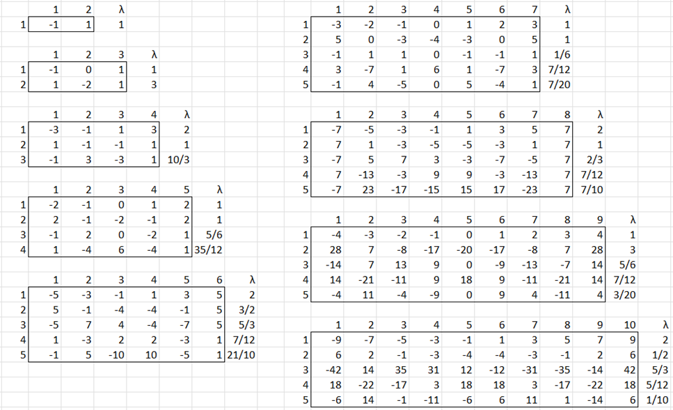
Figure 1 – Orthogonal Polynomial Contrast Coefficients
In the case where there are 5 equally-spaced treatments, the linear (1) coefficients from Figure 1 are -2, -1, 0, 1, 2, and the quartic (4) coefficients are 1, -4, 6, -4, 1. Note that since these are contrasts, the sum of the coefficients in any row is zero (e.g. 1-4+6-4+1 = 0). Since the contrasts are orthogonal, the product sum of any two rows in any one of these tables is also zero (e.g. -2(1)-1(-4)+0(6)+1(-4)+2(1) = 0). We will explain how to use the lambda values later.
Click here to learn about Real Statistics’ TREND_COEFF worksheet function that calculates the orthogonal polynomial contrast coefficients for you in Excel.
Polynomial contrast test
As explained in Planned Comparisons, for each type of trend (linear, quadratic, etc.), we use the contrast coefficients c1, …, ck for that trend. The test then becomes
 Thus
Thus

For a balanced model where n1 = n2 = … = nk = n, we have
Example
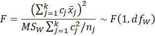
Example 1: Determine whether there is a significant linear, quadratic, cubic, and/or quartic trend for the data in Figure 2 based on drug dosages of 5, 10, 15, 20, and 25 mg.
Figure 2 – Data
We conducted an ANOVA using the Real Statistics Single Factor ANOVA data analysis tool. The results are shown in Figure 3.
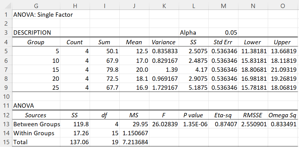
Figure 3 – ANOVA
We now partition the Treatment factor (Between Groups) as described above using the contrast coefficients for 5 treatment groups shown in Figure 1. The results are shown in Figure 4. Note that this analysis depends on the fact that the treatments (5, 10, 15, 20, 25) are equally spaced.
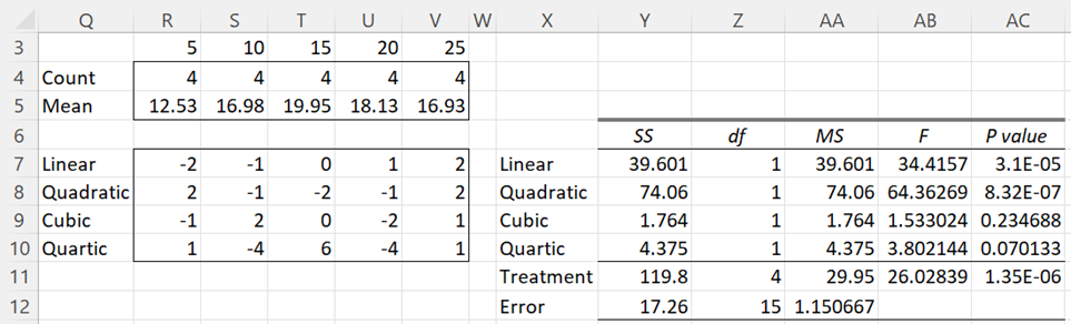
Figure 4 – Trend analysis
The count and means for each of the 5 treatment groups displayed in range R3:V5 are copied from range G5:H9 and J5:J9 of Figure 3. Also, the Treatment and Error values in range Y11:AC12 are copied from range H13:L14 of Figure 3. The contrast coefficients in range R7:V10 are copied from Figure 1.
The linear SS in cell Y7 is calculated via the array worksheet formula =SUMPRODUCT(R7:V7,R$5:V$5)^2/SUM(R7:V7^2/R$4:V$4). Highlighting the range Y7:Y10 and pressing Ctrl-D fills in the other SS values. The rest of the table is calculated using the usual formulas based on the error values in row 12. Note that the SS value in cell Y11 can be calculated by =SUM(Y7:Y10). A similar result holds for df.
Chart of the trends
We see that there are significant linear and quadratic trends. The cubic and quartic trends are not significant. This can also be seen from the chart shown in Figure 5 (the polynomial trendline is of degree 2).
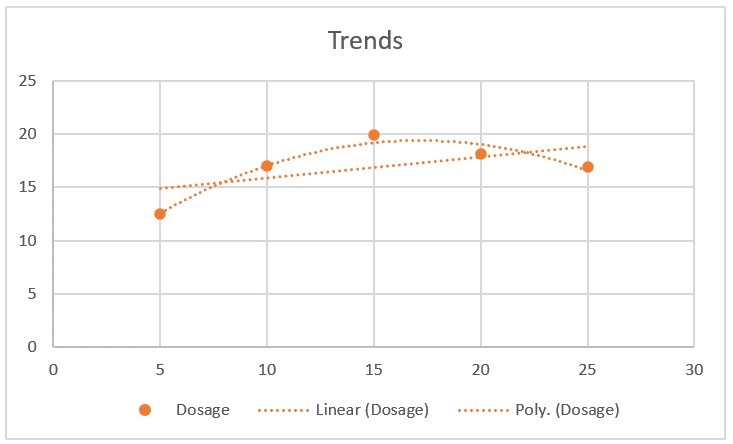
Figure 5 – Chart
Real Statistic Support
Real Statistic Function: The Real Statistic Resource Pack provides the following worksheet function.
TREND_ANOVA(R1, R2, sse, dfe, sst, lab): returns the ANOVA analysis using polynomial coefficients based on the group means in R1 and group counts in R2. sse is the error SS, dfe is the error df, and optionally sst, which is the treatment SS. If lab = TRUE (default FALSE), then row and column headings are appended to the output.
R1 and R2 are column arrays or ranges with the same number of rows. If the number of rows (i.e. the number of groups) k = 6, then Linear, Quadratic, Cubic, Quartic, and Quintic trend rows are output, followed by Treatment and Error rows.
The SS and df values for the Treatment row are equal to the sum of the values in SS and df values for the 5 types of trends. If k = 5, then no Quintic row is included, while if k = 4 then no Quartic or Quintic row is included. If k = 3 then no Cubic, Quartic, or Quintic row is included. R1 and R2 must have at least 3 rows. Note that for k = 3, 4, 5, or 6, the sst argument is not used and so can be omitted.
If k > 6, then the SS value for Treatment is set to the sst argument. df for Treatment is set to k-1, as expected. An extra row labeled “Other” is included just before the Treatment row which accounts for any polynomial trends whose degree is larger than 5.
We can obtain the output for Example 1, as shown in range X6:AC12 of Figure 4 (without the formatting) by using the array formula =TREND_ANOVA(J5:J9, H5:H9, H14, I14, , TRUE).
Examples Workbook
Click here to download the Excel workbook with the examples described on this webpage.
References
Bergerud, W. (1988) Determining polynomial contrast coefficients. Biometrics Information
No longer available online
Penn State University (2021) Orthogonal polynomials
https://online.stat.psu.edu/stat502/lesson/10/10.2
Howell, D. C. (2010) Statistical methods for psychology (7th ed.). Wadsworth, Cengage Learning.
https://labs.la.utexas.edu/gilden/files/2016/05/Statistics-Text.pdf
Fisher, R. A., Yates, F. (1963) Statistical tables, 6th ed. Macmillan Publishing
https://digital.library.adelaide.edu.au/dspace/handle/2440/10701
Anderson, R. L. (1942) Tables of orthogonal polynomial values extended to N=104
https://babel.hathitrust.org/cgi/pt?id=coo.31924000087100&seq=10
Horsley, R. (2022) Orthogonal polynomial contrasts individual df comparisons> equally spaced treatments.
No longer available online