In Dealing with Familywise Error, we describe some approaches for handling familywise errors. We now show how to apply these techniques when multiple t-tests are performed.
Example
Example 1: A school district uses four different methods of teaching their students how to read and wants to find out if there is a significant difference between the reading scores achieved using the four methods. A sample of students is randomly assigned to 4 classes, where each class uses a different one of the teaching methods. Based on the reading scores shown on the left side of Figure 1, determine whether there is a significant difference between the teaching methods.
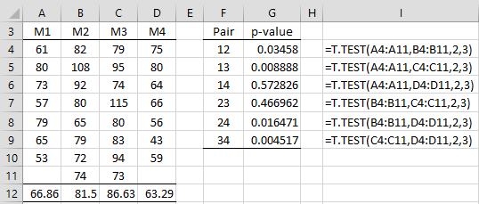
Figure 1 – Reading scores and pairwise t-tests
The mean scores for each method are shown in range A12:D12. There are C(4,2) = 6 pairs of methods, and so we can compare each pair to see whether there is a significant difference in the scores. This is shown on the right side of Figure 1.
Based on a significance level of .05, we see that pairs 12, 13, 24, and 34 yield a significant result. But as discussed Dealing with Familywise Error, this doesn’t account for familywise error. In fact, if we use a Bonferroni correction, then a familywise significance level of .05 becomes a significance level of .05/6 = .008333 for each test. In this case, the only significant comparison is 34, i.e. method 3 is significantly better than method 4 and we can’t say anything definitive about the other comparisons.
Multiple Test Data Analysis
This is a very conservative result. If we use the Benjamini-Hochberg option of the Multiple Tests data analysis tool (see Multiple Tests Analysis Tool) instead (with range F4:G9 in the Input Range), then as we can see from Figure 2, the pairs 34, 13, and 24 yield significant results.

Figure 2 – Benjamini-Hochberg test
ANOVA Follow-up
In Planned Comparisons , we explore more tailored approaches for dealing with familywise error for these sorts of situations, especially in conjunction with Analysis of Variance (ANOVA). In particular, we could use Tukey’s HSD test to determine which pairwise comparisons are significant. It turns out that the results from this test agree with our results from above, namely the pairs 34, 12, and 24 are significant.
In any case, we can use the Single Factor ANOVA data analysis tool to create the p-values shown on the right side of Figure 1. This is done by pressing Ctrl-m and selecting the Analysis of Variance option and then the ANOVA: Single factor from the dialog box that appears (or from the ANOVA tab when using the Multipage interface). In either case, fill in the dialog that appears as shown in Figure 3.
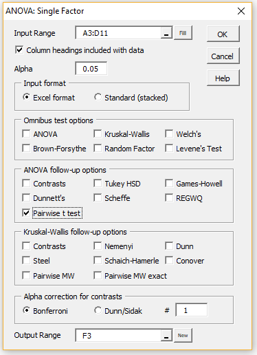
Figure 3 – Selecting the pairwise t-test option
Output
The output is shown on the left side of Figure 4. Note that the p-values as well as the mean differences are displayed for each of the 6 pairs.

Figure 4 – Pairwise t-tests
To obtain the Benjamini-Hochberg output shown on the right side of the figure, press Ctrl-m and select the Multiple Tests option (from the Misc tab if using the Multipage interface). When the dialog box shown in Figure 1 of Multiple Tests Analysis Tool appears enter F6:H11 in the Input Range (i.e. don’t include the column headings nor the mean column).
Examples Workbook
Click here to download the Excel workbook with the examples described on this webpage.
References
Howell, D. C. (2010) Statistical methods for psychology (7th ed.). Wadsworth, Cengage Learning.
https://labs.la.utexas.edu/gilden/files/2016/05/Statistics-Text.pdf
Wikipedia (2018) False discovery rate
https://en.wikipedia.org/wiki/False_discovery_rate
Charles
I believe that .05/6 = .00833, not .0833.
Hi Mark,
Thanks for catching this error. I have now made the correction.
I appreciate your help in improving the accuracy of the website and your ongoing support.
Charles