Confidence Interval for Coefficient of Variation

Basic Concepts

As shown in Measures of Variability, the coefficient of variation is defined as

where the formula on the left is the sample version and the formula on the right is the population version.

If V is the sample coefficient of variation, then this V is a biased estimate of the population coefficient of variation. In this case, an unbiased estimate of the population coefficient of variation is given by the formula

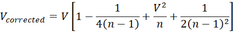
where n = the sample size. A shorter version is also commonly used, however, namely

Given a sample, we want to estimate a confidence interval for the population coefficient of variation based on the sample correlation of variation and the sample size. It turns out that there are many ways of creating such an estimate. We will consider four such approaches.

Kelley Estimate

This approach uses the noncentral t distribution.

First, we define

The Kelley confidence interval is

Naïve Estimate

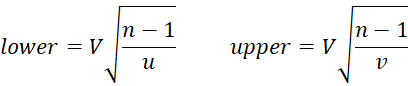
First, we define

The naïve confidence interval is then

McKay Estimate

The McKay confidence interval is

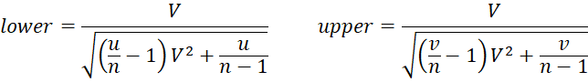
where u and v are as defined for the naïve estimate.

McKay’s estimate is valid for large values of n (at least n ≥ 10). McKay recommends this estimate only when the coefficient of variation is less than 0.33. Otherwise, McKay’s approximation may not be valid.

Vangel Estimate

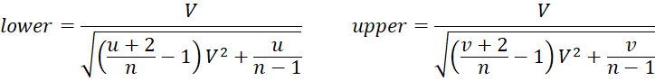
Vangel’s modification of McKay’s estimate gives better results for small samples but is still not recommended for V ≥ .33.

Worksheet Function

Real Statistics Function: The Real Statistics Resource Pack provides the following worksheet function.

CV_CONF(R1, lab, ctype, short, tails, alpha): returns a 4 × 1 column array with the values: CV of the data in R1, a corrected version of the CV, and the 1-alpha (default for alpha is .05) confidence interval for the CV.

If lab = TRUE (default FALSE) a column of labels is appended to the output. If short = TRUE (default) then the short version of the corrected CV is returned; otherwise, the long version is reported.

Which confidence interval is reported depends on the choice of ctype with values 1 (Kelley, default), 2 (Naïve), 3 (McKay) or 4 (Vangel). These are intervals around the sample V. You can also use the negative of these values, in which case the intervals are around the corrected version of V (short or long, depending on the value of short).

If tails = 2 (default) the two-tailed confidence interval (lower, upper) is returned. If tails = 1, then the two versions of the one-tailed confidence interval are (lower, ∞) and (-∞, upper).

Example

Example 1: Find the 95% confidence interval for the coefficient of variation based on the data in column A of Figure 1. Use the confidence intervals around the sample V (and not the corrected V).

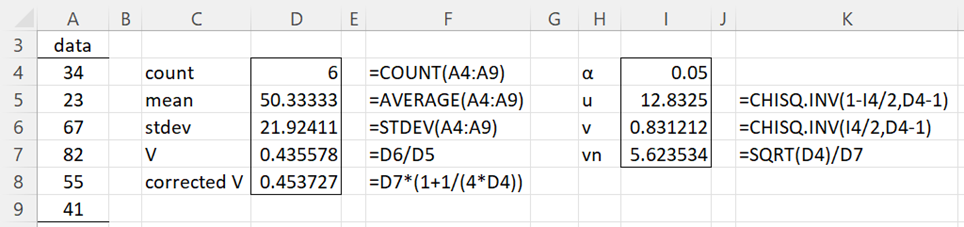
Figure 1 – CV confidence intervals (part 1)

In Figure 1 we report the shorter version of the corrected V in cell D8. If we had used the long version, then the formula in D8 would be =D7*(1+1/(4*D4)+D7^2/D4+1/(2*(D4-1)^2)).

Using the CV_CONF function, we obtain the estimates of the confidence interval shown in Figure 2.

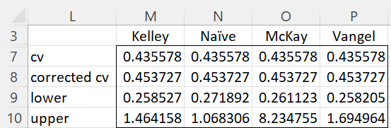
Figure 2 – CV confidence interval (part 2)

E.g. range L7:M10 contains the array formula =CV_CONF(A4:A9,TRUE), which is short for =CV_CONF(A4:A9,TRUE,1,TRUE, 2,.05). If we wanted to use the confidence interval around the long version of the corrected V, we would use the formula =CV_CONF(A4:A9,TRUE,-1,FALSE).

If we calculate the confidence interval manually using the Kelley estimate, we would insert the formula =SQRT(D4)/NT_NCP(I4/2,D4-1,I7) in cell M9 and =SQRT(D4)/NT_NCP(1-I4/2,D4-1,I7) in cell M10.

For the Vangel estimate we would use the formula =D7/SQRT(((I5+2)/D4-1)*D7^2+I5/(D4-1)) in cell P9 and =D7/SQRT(((I6+2)/D4-1)*D7^2+I6/(D4-1)) in cell P10. We could also use the Real Statistics array formula =CV_CONF(A4:A9,,4) in range P7:P10.

References

NIST Dataplot (2017) Coefficient of variation confidence limit
https://www.itl.nist.gov/div898/software/dataplot/refman2/auxillar/coefvari.htm 

Sokal, R. R. and Braumann, C. A. (1980) Significance Tests for coefficients of variation and variability profiles
https://academic.oup.com/sysbio/article-pdf/29/1/50/4659819/29-1-50.pdf

Beigy, M. (2019) Coefficient of variation
https://github.com/MaaniBeigy/cvcqv

McKay, A. T. (1932) Distributions of the coefficient of variation and the extended ‘t’ distribution. Journal of the Royal Statistical Society, Vol. 95, pp. 695-698.
https://www.jstor.org/stable/2342041

Vangel, M. (1996) Confidence intervals for a normal coefficient of variation. American Statistician, Vol. 15, No. 1, pp. 21-26.
https://www.jstor.org/stable/2685039

Forkman, J., Verrill, S. (2007) The distribution of McKay’s approximation for the coefficient of variation
https://www.fpl.fs.usda.gov/documnts/pdf2008/fpl_2008_forkman001.pdf