Basic Concepts
The t distribution characterizes how the t-test statistic is distributed when the null hypothesis is assumed to be true. The noncentral t distribution instead shows how the t-test statistic is distributed when the alternative hypothesis is assumed to be true (i.e. when the null hypothesis is assumed to be false). As such it is useful in calculating the statistical power and minimum sample size of the t-tests.
Definition
Definition 1: The noncentral t distribution, abbreviated as T(k,δ) has the following cumulative distribution function F(t), written as Fk,δ(t) when necessary, where k = the degrees of freedom and δ = the noncentrality parameter.

when t ≥ 0, where Φ is the cumulative distribution function of the standard normal distribution, i.e.
Φ(z) = NORM.S.DIST(z, TRUE)
and Ir(a,b) is the cumulative distribution function of the beta distribution
Ir(a,b)= BETA.DIST(r,a,b, TRUE)
where
![]()
Algorithm for cdf
We can express the pdf of the Poisson distribution with mean λ as
![]() Thus
Thus![]()
and so we can express the cdf of the noncentral t distribution as
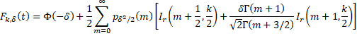
where Γ(k) is the gamma function. Since Γ(m+1)/Γ(m+3/2) can be expressed by the formula =EXP(GAMMALN(m+1)-GAMMALN(m+3/2)), the cdf of the noncentral t distribution can be expressed in Excel as a finite sum of terms using POISSON.DIST, BETA.DIST, NORM.S.DIST, and GAMMALN.
The more terms used in the finite sum, the better the precision, although, after a certain point, overflow errors will be encountered. For this reason, the Real Statistics functions described below use a bit more sophisticated approach.
When t < 0, the noncentral t distribution is defined as
![]()
Algorithm for pdf
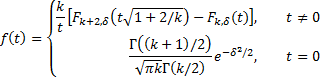
We can calculate the probability density function (pdf) of the noncentral t distribution as follows:
Characteristics
The mean and variance of the distribution are
![]()
![]()
The shape of the noncentral t distribution is similar to that of the central t distribution (i.e. the ordinary t distribution). The noncentrality parameter indicates how much the distribution is shifted to the right (when δ > 0) or to the left (when δ < 0). When δ = 0, the noncentral t distribution is identical to the central t distribution, and so T(k,0) = T(k).
Graphs
The chart in Figure 1 shows the graphs of the noncentral t distribution with 10 degrees of freedom for δ = 0, 2, 4, and 6.
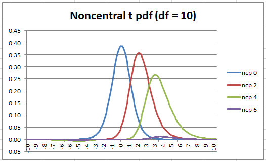
Figure 1 – Noncentral t pdf by noncentrality parameter
The chart in Figure 2 shows the graphs of the noncentral t distribution with δ = 2 and the degrees of freedom = 1, 3, 5, 10.
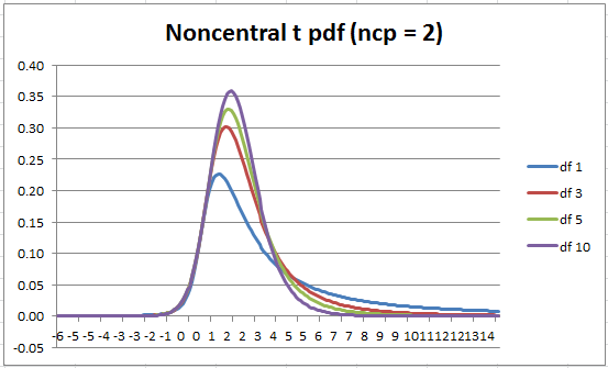
Figure 2 – Noncentral t pdf by degrees of freedom
Worksheet Functions
Real Statistics Functions: The Real Statistics Resource Pack supplies the following worksheet functions:
NT_DIST(t, df, δ, cum, iter, prec). If cum = TRUE then the value of the noncentral t distribution T(k,δ) at t is returned, while If cum = FALSE then the value of the noncentral pdf at t is returned.
NT_INV(p, df, δ, iter, iter0, prec) = the inverse of the cdf of the noncentral t distribution T(k,δ) at p, i.e. the value of t such that NT_DIST(t, df, δ, TRUE, iter, prec) = p.
NT_NCP(p, df, t, iter, iter0, prec) = the value of the noncentrality parameter δ such the cdf of the noncentral distribution T(k,δ) at t is p, i.e. NT_DIST(t, df, δ, TRUE, iter, prec) = p.
Here iter = the maximum number of terms from the infinite sum (default 1000) and prec = the maximum amount of error acceptable in the estimate of the infinite sum unless the iteration limit is reached first (default = 0.000000000001). iter0 = the number of iterations used in calculating NT_INV or NT_NCP by binary search (default 40).
Note that NT_DIST(4.5,10,4,FALSE) = .25497 and NT_DIST(4.5,10,4,TRUE) = .60368, which is consistent with the values shown in the green curve of Figure 1.
Examples Workbook
Click here to download the Excel workbook with the examples described on this webpage.
References
Steier, J. F. and Fouladi, R. T. (1997) Noncentrality interval estimation and the evaluation of statistical models
http://www.statpower.net/Steiger%20Biblio/Steiger&Fouladi97.PDF
Scholz, F. W. (2008) Applications of the Noncentral t-Distribution
https://faculty.washington.edu/fscholz/DATAFILES498B2008/NoncentralT.pdf
Krishnamoorthy, K. (2006) Handbook of statistical distributions with applications. Chapman and Hall
https://www.academia.edu/41846183/Handbook_of_Statistical_Distributions_with_Applications
Benton, D. and Krishnamoorthy, K. (2003) Computing discrete mixtures of continuous
distributions: noncentral chisquare, noncentral t and the distribution of the square of the sample multiple correlation coefficient. Computational Statistics & Data Analysis 43. 249 – 267
https://papers.ssrn.com/sol3/papers.cfm?abstract_id=3142698
Hello
I was using the Noncentral t and F functions. Maybe you can explain something. When I review the relation between the F() and t() distribution functions with noncentrality (d) = 0, the Probability for the F(x,1,v2, true) [d = 0] will equal (1+t(x^0.5, v2, true))/2. For example, F(9,1,4,true) = 0.960058, and the t(9^0.5, 4, true) = 0.980029. And (1 + F()) / 2 = 0.980029. So this holds for d = 0
However, in Abramowitz and Stegan’s book (Handbook of Mathematical Functions, Eq. 26.6.19), they show the relationship between the F and t-Distribution with a nonzero noncentrality parameter (d) to be given by:
F(x,1,v2,true,d) = t(x^0.5, v2, true, d^0.5)
All I can find in the references is that this relation “holds” for all values of d.
I ran the calculations for various d {0…11) using your spreadsheet and found that for small values of d (i. e. d = 1), the relation does not hold, but as d increases, the values converge to the relationship.
Nf_Dist(9,1,4,TRUE,1) = 0.899141 nt_dist(3,4,True,1) = 0.934475. Delta = 0.00218
Nf_Dist(9,1,4,TRUE,3) = 0.772714 nt_dist(3,4,True,1.73205081) = 0.772991. Delta = 0.00028
Etc.
It appears that as “d” increases the values converge to the Abramowitz relation defined in equation 26.6.19.
Maybe I did something wrong, but do you confirm this, and is there an explanation as to why this relation does not hold for small noncentrality parameters and “converges” at higher values?
Thanks!
Dan
Hi Dan,
I just used the calculators at https://keisan.casio.com/exec/system/1180573219 and https://keisan.casio.com/exec/system/1180573165, and I obtained the same values that I got from the Real Statistics functions, namely NF_Dist(9,1,4,1,TRUE) = 0.899141 and NT_Dist(3,4,1,TRUE) = 0.901321.
Thus, the equivalence doesn’t hold for small values of ncp. In fact, if ncp = 0 then from your above calculations
F(9,1,4,true) = 0.960058 and T(9^0.5, 4, true) = 0.980029, which are not equal. If instead of ncp = 0, you use some small value such as .0001, you will see similar values.
I note that this equivalence is also claimed at https://en.wikipedia.org/wiki/Noncentral_t-distribution
Charles
Hi Charles
I want to use the NT_INV function to calulate the deviate t (also called the tolerance factor k) with both probability and confidence 95% for incresing df.
The NT_INV(0.95;df;1.6445) provides me with the following results
df NT_INV k95,95
2 26.5460546 26.26
3 8.377973059 7.655
4 5.9566958 5.145
5 5.076619865 4.202
6 4.62913949 3.707
7 4.359690547 3.399
8 4.180055166 3.188
9 4.051878325 3.031
10 3.955872695 2.911
1000 3.294991017
10000 3.29023463
100000 3.289759982
1000000 3.289712527
10000000 3.289707781
100000000 3.289707307
1000000000 3.289707259
10000000000 3.289707254
1E+11 3.289707254
1E+12 3.289707254
1E+13 3.289707254
1E+14 3.289707254 1.6448
At the right the expected k95,95 tolerance limits as found in the handbooks.
The NT_INV does not asymptotically go to 1.6448 for df->infinity as would be expected.
Am I doing something wrong? Or is it a bug?
It seems to be going to twice 1.6445.
Charles
Dear Charles
Indeed, it seems twice the expected value.
My colleague tried it as well and came to the same results.
I’ve tried to work with adapted df, but that made it even worse.
Are you able to solve it? I can send you the VB6 algorithm I use in the Hyginist program (http://www.tsac.nl/hyginist.html)
Maybe my lay-out was confusing
N NT_INV literature
2 26.5460546 26.26
3 8.377973059 7.655
4 5.9566958 5.145
5 5.076619865 4.202
inf. 3.289707254 1.6445
A colleague suggested to use in EXCEL =NT_INV(NT_DIST;df;NORM.S.INV(p)*SQRT(N))/SQRT(N)
so with p the desired probability, the value of the noncentrality parameter δ=NORM.S.INV(NT_DIST)*SQRT(N) and NT_DIST the desired confidence.
And than devide the resulting NT_INV() by SQRT(N)
This results in δ which corresponds with the tables in literature
Please confirm this is the right approach
Theo,
I don’t know whether this is the right approach.
Charles
Hello Charles,
I was looking at your “CI Functions for Effect Size d” article, and I cannot find the NT_NCP function (Noncentral t Distribution) on Excel (version 16.54). I need to calculate Confidence Intervals for Cohen’s d when only means and their standard deviations of two groups are given.
What should I do about this?
Hello Pauline,
NT_NCP is not a standard Excel function. It is provided by the Real Statistics Resource Pack. You can download this Excel add-in for free. Once you do that, you can use NT_NCP (and many other statistics functions) just like any other Excel function.
You can download Real Statistics from
https://www.real-statistics.com/free-download/real-statistics-resource-pack/
Charles
Hello Charles,
I left a post on this topic already but may have done so on the wrong page and have simplified the question a bit. It seems more appropriate to post here:
Some texts and websites state the non-central t can be used to estimate confidence intervals of percentiles. For instance, the left -3 sigma tail of a standard Normal distribution has area = 0.00135 or 0.135% and the following Matlab command illustrates what is supposed to work to find the left 95% confidence tail (2.5% cumulative area) for the 0.135% tail if sampled many times (10 million) with 10,000 samples each:
n=10^4
Z=-3.00
C=-1.96
[nctinv(1-normcdf(C,0,1), n-1, -1*sqrt(n)*Z) * 1 / sqrt(n), nctinv(normcdf(C, 0,1), n-1, -1*sqrt(n)*Z) * 1/sqrt(n)]
NonCentrality Parameter = Delta / [Sigma/Sqrt(n)] = Z*Sqrt(n) = -3*Sqrt(n)
StdErrorOfEstimateForMean = SEM = 1/Sqrt(n) and texts use this value.
This produced (-3.0466, -2.9546) which is too narrow.
And Hald (1952) shows a formula that works very well and Matches Monte Carlo:
Variation = 1/NORM.DIST(-3,0,1,FALSE)^2*NORM.DIST(-3,0,1,TRUE)*(1-NORM.DIST(-3,0,1,TRUE))/10000.
(It also worked for the 95% limits of the 95% tails and the 95% limits for the Median)
StdDev = Sqrt(Variance)
Left 95% Tail Of 0.135% Percentile = -3 – 1.96 * StdDev = -3.1624 (MC showed -3.17)
Right 95% Tail Of 0.135% Percentile = -3 + 1.96 * StdDev = -2.8376 (MC showed -2.84)
Can you please show how to properly use the noncentral t to get similar results, especially using Excel for the non-central as you did for other problems?
Thanks,
Bruce
Hello Bruce,
I responded to your earlier comment yesterday. I repeat my response as follows.
Thank you for your kind words about the Real Statistics website.
From your comment, I understand that the simulation that you are proposing is based on the non-central t distribution.
The Real Statistics software supports the non-central t distribution. In particular, it provides the inverse function NT_INV(p, df, ncp).
For any given value of df and ncp, you can obtain a random value from the stated non-central t distribution by using the formula
=NT_INV(RAND(), df, ncp)
You can then generate as many random values as you like and estimate the desired parameter(s) and get confidence intervals. I don’t know a priori how big a sample is required to achieve the accuracy that you are looking for, but the good news about Monte Carlo simulations is that you can estimate the confidence interval and with a little experimentation you should be able to make an educated guess to the sample size required.
I don’t know of a closed-form solution, but perhaps the Real Statistics function =NT_DIST(x,df,ncp,cum) could be useful.
Charles
Charles,
What does the “t” stand for in NT_DIST(t, df, sigma, cum, m).
Is it the Tstat derived from the problem? # of tails? You never specify.
Also, if it’s the Tstat derived from the problem, from what I can tell this ought to be the same as the NCP, which most of the time will give an answer of approximately 0.5.
Thank you
Or rather, if you use the same value for t and sigma in the NT_DIST function then it will usually give an answer that’s approximately 0.5.
Okay, sorry if I’m overcrowding things here, but upon further inspection it looks like if you use the 2-tailed Tcrit for the NT_DIST function this gives answers that are almost identical to the statistical power option in the RealStats plug in.
Am I correct here?
Thanks.
Jonathan,
The formula is NT_DIST(t, df, ncp, cum, m), where ncp is the noncentrality parameter. The t is the same as the t in T.DIST(t,df,cum). In fact, when ncp = 0 then NT_DIST(t,df,0,cum) = T.DIST(t,df,cum).
Charles
Hi, Charles
I have tried to use the function NT_INV for the purpose of calculating one-side tolerance intervals, with the parameters p=0.95, df=50, delta=11.63, m=170. It did not provide a solution. Actually it did not work with df larger than 50 and delta larger than 11. Please help.
Sam
Sam,
Some observations:
1. For some values of p, df and delta the value for m must be less than 170. E.g. for your example, if you change m = 170 to m = 168, the function will generate the correct answer. I need to improve the function to avoid this problem.
2. There are solutions for values of df larger than 50 or delta larger than 11. E.g. NT_INV(.95,60,12,165) = 14.79959488, NT_INV(.95,100,12,150) = 14.3688301.
3. But the function doesn’t seem to be able to find all such solutions. E.g. NT_INV(.95,60,20,m) does not find the right value, which I believe is about 24. I need to fix this.
Thanks for identifying this problem.
Charles
Thanks, Charles.
Sam
Hi,
I have the following doubt about this distribution:
How small should we consider t to calculate the pdf as t=0. For example, if we have t=1E-10 and use the algorithm for x not zero we ca<n introduce a distortion in the graphic that bis noticeable in certain cases. We can say that the second algorithm must be used not only for t=o but 'in the vicinity of 0'.
Did you felt this this probçem and Have you any idea of how to define its limits?
António Teixeira
António,
Excellent point. I have checked the pdf values for t = E-5, E-6, E-7, E-8, E-9, E-10, 0 with df = 1 to 20 and ncp = 4, 3, 2, 1, .5, .1, .01, all carried out to 8 decimal places.
For ncp = 3, the value at t = 0 is always the same as the value at E-9. For 7 values of df the pdf values at t = E-10 is higher than that at t = E-9 (this theoretically shouldn’t happen), the difference is at most .00000003. For 5 values of df the pdf value at t = E-10 is lower than that at t = E-9, the difference is at most .00000002.
For the other values of ncp, usually the pdf value at t = 0 is equal to that of t = E-8, E-9 or somewhere in between, although occasionally at E-7. There seems to be more distortion at E-10 where fairly often the pdf value at E-10 is higher than at E-9, although sometimes this starts to happen (although not for all values of df) at E-9 or E-8.
Based on this analysis, I would say that for ncp >= 1 the second value of the pdf could be used for t < E-8. For ncp < 1 perhaps this should be for t < E-7.
Charles