Kolmogorov-Smirnov Test for Normality

Hypothesis Testing

Definition 1: Let x₁,…,x_n be an ordered sample with x₁ ≤ … ≤ x_n and define S_n(x) as follows:

Now suppose that the sample comes from a population with cumulative distribution function F(x) and define D_n as follows:

Observation: It can be shown that D_n doesn’t depend on F. Since S_n(x) depends on the sample chosen, D_n is a random variable. Our objective is to use D_n as a way of estimating F(x).

Critical Values

The distribution of D_n can be calculated (see Kolmogorov Distribution), but for our purposes now the important aspect of this distribution is the table of critical values. These can be found in the Kolmogorov-Smirnov Table.

If D_n,α is the critical value from the table, then P(D_n ≤ D_n,α) = 1 – α. D_n can be used to test the hypothesis that a random sample came from a population with a specific distribution function F(x). If

then the sample data is a good fit with F(x).

Confidence Interval

Also from the definition of D_n given above, it follows that

Thus S_n(x) ± D_n,α provides a confidence interval for F(x)

Examples (Frequency Table)

Example 1: Determine whether the data represented in the following frequency table is normally distributed where x represents rainfall amounts.

Figure 1 – Frequency table for Example 1

This means that 8 elements have an x value less than 100 (i.e. between 0 and 100), 25 elements have an x value between 101 and 200, etc. We need to find the mean and standard deviation of this data. Since this is a frequency table, we can’t simply use Excel’s AVERAGE and STDEV functions. Instead, we first use the midpoints of each interval and then use an approach similar to that described in Frequency Tables as shown in Figure 2:

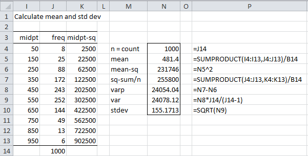
Figure 2 – Calculating mean and standard deviation

Thus, the mean is 481.4 and the standard deviation is 155.2. We can now build the table that allows us to carry out the KS test, as shown in Figure 3.

Figure 3 – Kolmogorov-Smirnov test for Example 1

Columns A and B contain the data from the original frequency table. Column C contains the corresponding cumulative frequency values and column D simply divides these values by the sample size (n = 1000) to yield the cumulative distribution function S_n(x)

Column E uses the mean and standard deviation calculated previously to standardize the values of x from column A. E.g. the formula in cell E4 is =STANDARDIZE(A4,N$5,N$10), where cell N5 contains the mean and cell N10 contains the standard deviation (from Figure 2). Column F uses these standardized values to calculate the cumulative distribution function values assuming that the original data is normally distributed. E.g. cell F4 contains the formula =NORM.S.DIST(E4,TRUE). Finally, column G contains the absolute values of the differences between the values in columns D and F. E.g. cell G4 contains the formula =ABS(F4—D4). If the original data is normally distributed these differences will be zero.

Test Results

Now D_n = the largest value in column G, i.e. MAX(G4:G13) = 0.0117 (cell G8). If the data is normally distributed then the critical value D_n,α will be larger than D_n. From the Kolmogorov-Smirnov Table we see that

D_n,α = D_1000,.05 = 1.36 / SQRT(1000) = 0.043007

Since D_n = 0.0117 < 0.043007 = D_n,α, we conclude that the data is a good fit for the normal distribution.

Example (Raw Data)

Example 2: Using the KS test, determine whether the data in Example 1 of Graphical Tests for Normality and Symmetry is normally distributed.

We follow the same procedure as in the previous example to obtain the results shown in Figure 4. Since the frequencies are all 1, this example might be a little easier to understand.

Figure 4 – KS test for data from Example 2

The Kolmogorov-Smirnov Table shows that the critical value D_n,α = D_15,.05 = .338.

Since D_n = 0.1874988 < 0.338 = D_n,α, we conclude that the data is a reasonably good fit with the normal distribution. This is inconsistent with the QQ plot shown in Figure 5, which seems to show that the data is not normally distributed.

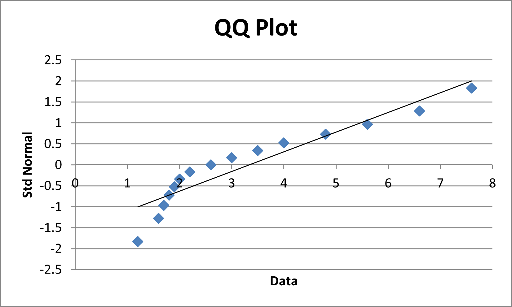
Figure 5 – QQ Plot for Example 2

The reason for this inconsistency is that the Kolmogorov-Smirnov test in the form presented above is only valid when the population mean and standard deviation are known, and not estimated from the sample. In the case where the population mean and standard deviation are not known, you need to use the Lilliefors version of the test, as described below.

Worksheet Functions

Real Statistics Functions: The following functions are provided in the Real Statistics Resource Pack:

KSCRIT(n, α, tails, interp) = the critical value of the Kolmogorov-Smirnov test for a sample of size n, for the given value of alpha (default = .05) and tails = 1 (one tail) or 2 (two tails, default), based on the KS Table. If interp = TRUE (default) then the recommended interpolation is used; otherwise, linear interpolation is used.

KSPROB(x, n, tails, iter, interp, txt) = an approximate p-value for the KS test for the D_n value equal to x for a sample of size n and tails = 1 (one tail) or 2 (two tails, default) based on a linear interpolation (if interp = FALSE) or recommended interpolation (if interp = TRUE, default) of the values in the Kolmogorov-Smirnov Table, using iter number of iterations (default = 40).

Note that the values for α in the Kolmogorov-Smirnov Table range from .001 to .2 (for tails = 2) and .0005 to .1 for tails = 1. When txt = FALSE (default), if the p-value is less than .001 (tails = 2) or .0005 (tails = 1) then the p-value is given as 0, and if the p-value is greater than .2 (tails = 2) or .1 (tails = 1) then the p-value is given as 1. When txt = TRUE, then the output takes the form “< .001”, “< .0005”, “> .2” or “> .1”.

For Example 2, KSCRIT(15, .05, 2) = .338 (the same as shown in cell H21 of Figure 4). Also note that the p-value = KSPROB(H20, B21) = KSPROB(0.184177, 15) = 1 (meaning that p-value > .2), and so once again we can’t reject the null hypothesis that the data is normally distributed.

If the value of D_n had been .35 in Example 2, then D_n = .35 > .338 = D_crit, and so we would have rejected the null hypothesis that the data is normally distributed. In this case, we would have seen that p-value = KSPROB(.35,15) = .0427, which once again leads us to reject the null hypothesis.

Kolmogorov Distribution

As referenced above, the Kolmogorov distribution can be useful in conducting the Kolmogorov-Smirnov test. Click here for more information about this distribution, including some useful functions provided by the Real Statistics Resource Pack.

Lilliefors Test

When the population mean and standard deviation for the Kolmogorov-Smirnov Test is estimated from the sample mean and standard deviation, as was done in Example 1 and 2, then the Kolmogorov-Smirnov Table yields results that are too conservative. More accurate results can be derived from the Liiliefors Table as described in the Lilliefors Test for Normality.

References

National Institute of Standards and Technology NIST (2021) Kolmogorov-Smirnov goodness-of-fit test
https://www.itl.nist.gov/div898/handbook/eda/section3/eda35g.htm

Wikipedia (2012) Kolmogorov-Smirnov test
https://en.wikipedia.org/wiki/Kolmogorov%E2%80%93Smirnov_test