Comparing Logistic Regression Models

Full logistic regression model

Example 1: Repeat the study from Example 3 of Finding Logistic Regression Coefficients using Newton’s Method based on the summary data shown in Figure 1.

Figure 1 – Data for Example 1

Press Ctrl-m and select the Logistic and Probit Regression data analysis tool, (from the Reg tab if using the Multipage interface). Fill in the dialog box that appears as shown in Figure 2.

Figure 2 – Logistic Regression dialog box

After clicking on the OK button, the output shown in Figure 3 is displayed.

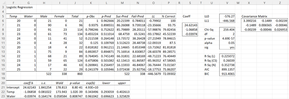
Figure 3 – Base model for Example 1

We know from the above analysis that the presence of Temp and Water makes a significant difference (over the initial model where only the intercept is used), but do we need both of these independent variables? 1 = exp(0) doesn’t lie in the 95% confidence interval for Temp, but it does lie in the 95% confidence interval for Water. We conclude that Temp makes a significant contribution to the model, but Water doesn’t. Since this analysis relies on the Wald statistic, which is not completely reliable, we would prefer to use an approach similar to that used in Testing Fit of the Logistic Regression Model.

Reduced model

Example 2: Do the Temp and Water variables make a significant difference in the model of Example 1?

We first create summary tables for the Temp-only and Water-only models and then use the Logistic Regression data analysis tool (with the Newton option) to build the two models. We can do this by using one of the following Real Statistics functions.

Worksheet Functions

Real Statistics Functions: The Real Statistics Resource Pack provides the following array functions where R1 contains data for a logistics regression model in summary form.

LogitSelect(R1, s, head) – array function which takes the summary data in range R1 and outputs an array in summary form based on s. If head = TRUE then column headings are included in R1 as well as in the output. The string s is a comma-delimited list of independent variables in R1 and/or interactions between such variables. E.g. if s = “2,3,2*3” then the data for the independent variables in columns 2 and 3 of R1 plus the interaction between these variables are output.

LogitReduce(R1, s) – array function that takes summary data in R1, including column headings, and fills the highlighted range with the data in R1 omitting the columns described by the string s, where s is a comma delimited list of column headings in R1

Temperature-only model

Example 2 (continued): The summary table for the Temp-only model is shown in range A27:C33 of Figure 4. This is created by inserting the array formula =LogitSelect(A3:D15,”1”,TRUE) in range A27:C33 and then pressing Ctrl-Shft-Enter. Alternatively, we can use the array formula =LogitReduce(A3:D15,”Water”).

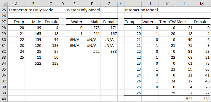
Figure 4 – Reduced and interaction models

Note that when creating the summary table for the Temp-only, you just need to make sure that you highlight a sufficient number of rows to contain all the data. If you highlight more rows than are necessary, these extra rows will be filled with #N/A values; you won’t include these extra rows when specifying the Input Range in the dialog box of the Logistic/Probit Regression data analysis tool (shown in Figure 2) when analyzing the Temp-only model.

Output

We now use the Logistic/Probit Regression data analysis tool (choosing the Logistic option and placing A27:C33 in the Input Range) to obtain the output shown in Figure 5.

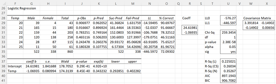
Figure 5 – Output for Temp-only model

We observe that the Temp variable makes a significant contribution (cell U35) over the constant-only model. Here we are comparing LL1 (Temp model) with LL0 (constant-only model).

We can also compare the Temp model with the base model (Temp + Water), by first copying the range T28:U35 to another location in the worksheet (W53:X60, as shown in Figure 6). Next, we place the formula =U6 in cell X54 (i.e. the LL1 value from the base model) and =U29 in cell X53 (substituting the LL1 value from the Temp model for LL0). We also need to change df to 1 (in cell X57) since the difference between the df of the two models is 2 – 1 = 1. The result is shown in Figure 6.

Figure 6 – Comparing the Temp and base models

We see there is not a significant difference between the models (cell X60). This confirms the conclusion that we reached previously that the Water variable is not making a significant contribution, and in fact, it can be dropped.

Water-only model

You can create the Water-only model in a similar way, using either the array formula =LogitSelect(A3:D15,”2”,TRUE) or =LogitReduce(A3:D15,”Temp”), to obtain the output shown in range E27:G29 of Figure 4.

Using the Logistic/Probit Regression data analysis tool (placing E27:G29 in the Input Range), we obtain the output shown in Figure 7.

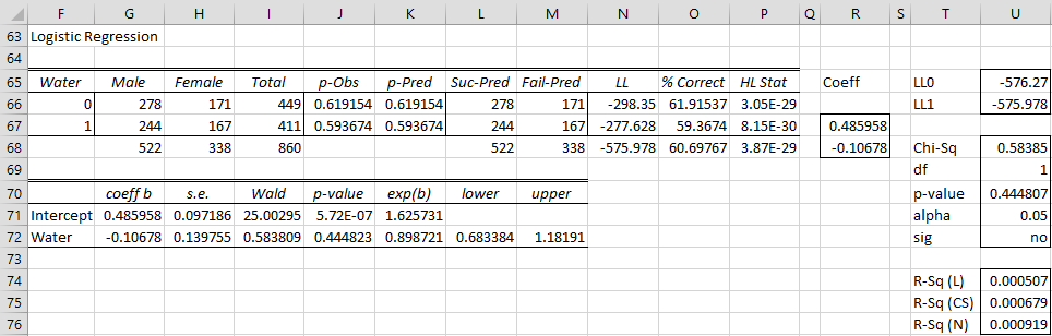
Figure 7 – Output for Water-only model

This time we see that there is no significant difference between the Water model and the constant model. If we repeat the analysis of Figure 6, we see there is a significant difference between the Water model and the base model, as shown in Figure 8.

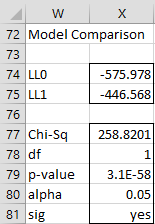
Figure 8 – Comparing the Water-only and base models

This confirms, once again, that the Temperature is making a significant contribution to the model.

Note that we can’t compare the Water-only and Temp-only models in this way since neither is a subset of the other.

Interaction model

Finally, we can look at further refinements of the model, such as the full interaction model, where we include the interaction between Temp and Water. We first create the data for this model by highlighting the range I27:M39 (shown in Figure 4), inserting the formula =LogitSelect(A3:D15,”1,2,1*2”,TRUE), and pressing Ctrl-Shft-Enter.

We now use the Logist/Probit Regression data analysis tool on the data in I27:M39 to obtain the analysis shown in Figure 9 (with the covariance matrix shown on the upper part of Figure 10).

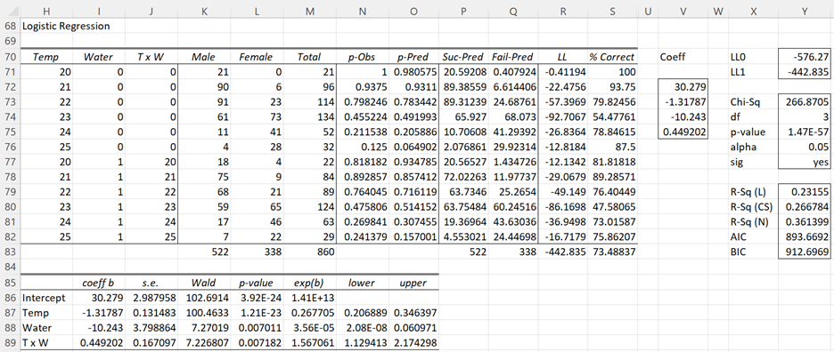
Figure 9 – Logistic regression – Interaction model

If we compare this model with the base model using the approach described above, we get the output shown in Figure 10.

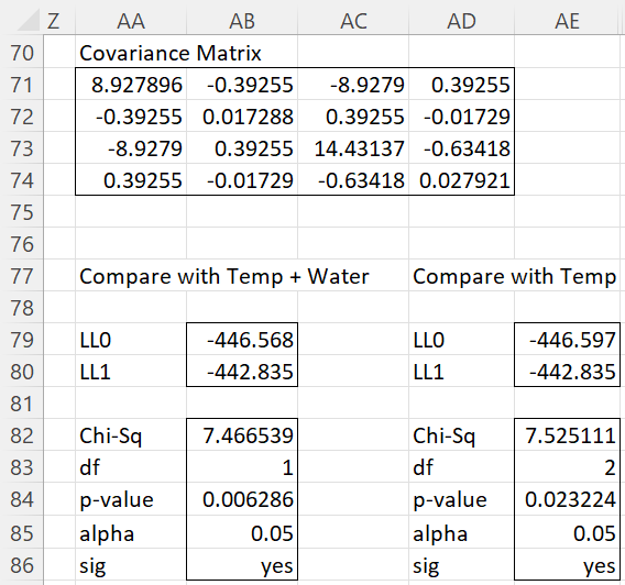
Figure 10 – Comparing the interaction and base models

Figure 10 shows there is a significant difference between the full interaction model and the base model, with the interaction model providing a better fit.

Examples Workbook

Click here to download the Excel workbook with the examples described on this webpage.

References

Howell, D. C. (2010) Statistical methods for psychology (7^th ed.). Wadsworth, Cengage Learning.
https://labs.la.utexas.edu/gilden/files/2016/05/Statistics-Text.pdf

Christensen, R. (2013) Logistic regression: predicting counts.
http://stat.unm.edu/~fletcher/SUPER/chap21.pdf

Wikipedia (2012) Logistic regression
https://en.wikipedia.org/wiki/Logistic_regression

Agresti, A. (2013) Categorical data analysis, 3rd Ed. Wiley.
https://mybiostats.files.wordpress.com/2015/03/3rd-ed-alan_agresti_categorical_data_analysis.pdf