Weibull with Multi-Censored Data

Basic Concepts

In Weibull with Censored Data, m+n components enter into service at time 0 and n components fail at various times before time t. x₁, …, x_n units of time, and m components stay in service for (at least) y₁, …, y_m units of time. 

We now consider the case where n components fail after x₁, …, x_n units of time, and m components stay in service for y₁, …, y_m units of time. In this scenario, the components don’t all need to go into service at the same time. Also, some of the components can be removed from service at various times without failing.

The likelihood function now takes the form

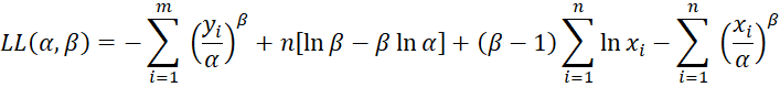
where f(x) is the pdf of a distribution and F(x) is the cdf of that distribution. The log-likelihood function is

For the Weibull distribution

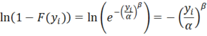
Thus

Optimization

We can use Solver to find the values of α and β that maximize LL(α,β). Alternatively, we can use Newton’s method based on the extension to the iterative approach described in Fitting Weibull Parameters via MLE and Newton’s Method when there is no censored data.

Step 0: make an initial guess β₀ for the value of β.

Step k+1: Assuming that we have an estimate  of β_k, we define a new estimate β_k+1, that should be more accurate, as follows:

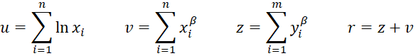
where

and

This process is repeated until the value of β_k converges, at which point we calculate the alpha parameter by

Convergence occurs when h(β_k) is close to zero or β_k+1 ≈  β_k.

We won’t give an example of the use of these steps, although the approach is similar to that used for Example 1 of Weibull with Censored Data. Instead, we will give two examples using the following Real Statistics functions.

Worksheet Functions

Real Statistics Functions: The Real Statistics Resource Pack provides the following functions where R1 is a column array containing the x₁, …, x_n values, R2 is a two-column array in the form of a frequency table containing the y₁, …, y_m values. lab, iter, and bguess are as for the WEIBULL_FIT function (see Weibull with Censored Data). viter is the number of iterations used to calculate, by simulation, the variance of the data (including censored values). viter defaults to zero (meaning that this variance is not calculated).

WEIBULL_MCFIT(R1, R2, lab, iter, bguess, viter):  returns an array with the Weibull distribution parameter values alpha and beta, the actual and estimated mean and variance, and MLE  based on the data in the column range R1 plus the estimated mean time to failure of the censored data elements

There are also the following non-array functions:

WEIBULL_MCMEAN(R1, R2, alpha, beta) = the mean of all the data in R1 plus the average life of the censored data in R2 based on a Weibull distribution with parameters alpha and beta

WEIBULL_MCVAR(R1, R2, alpha, beta, iter) = the variance of all the data in R1 as well as an estimate of the variance of the censored data in R2 using iter simulations (default 20,000) from a Weibull distribution with parameters alpha and beta

We can use the WEIBULL_MCFIT function to give the results for Example 1 of Weibull with Censored Data, as shown in columns F and G of Figure 1.

Figure 1 – Multi-censored fit

We insert the array formula

=WEIBULL_MCFIT(A4:A15,F4:G4,TRUE,,,20000)

in range F6:G12 to obtain the results that are identical to those in range L15:M21 of Figure 1 of Weibull with Censored Data with the exception of a slightly different actual variance estimate that is based on a simulation.

Example

Example 1: Repeat Example 1 of Weibull with Censored Data using the censored data shown in the frequency table in range I3:J6 of Figure 1.

Once again two components go into service at time t = 0 but have not failed at time t = 900. In addition, there is one component that stayed in service for 400 hours and another 3 that stayed in service for 100 hours.

It doesn’t matter whether the component that stayed in service for 400 hours came into service at time t = 0 and then was removed from service at time t = 400 without failing or came into service at time t = 500 and then hadn’t failed at time t = 900. In fact, this component could have come into service at any time between t = 0 and t = 500, as long it only remained in service for 400 hours without failing.

The situation is similar for the 3 components that remained in service for 100 hours. In fact, one of these components could have been put into service at t = 0 and removed at t = 100, another could have been put in service at t = 200 and removed at t = 300 and the third could have been put into service at t = 800 and removed at t = 900.

Using the array formula =WEIBULL_MCFIT(A4:A15,I4:J6,TRUE,,,20000) we get the results shown in range I8:J14.

Examples Workbook

Click here to download the Excel workbook with the examples described on this webpage.

Reference

EpiX Analytics (2018) Using optimization to maximize a likelihood calculate to obtain MLEs
https://modelassist.epixanalytics.com/display/EA/Using+optimization+to+maximize+a+likelihood+calculation+to+obtain+MLEs