Fitting GEV Distribution via MLE

Basic Approach

The likelihood function for a sample {x₁, …, x_n} from a Generalized Extreme Value (GEV) distribution with parameters μ, σ and ξ is

where

Thus

Let z_i = (x_i – μ)/σ and y_i = 1 + ξz_i. Thus

and so the log-likelihood function is

Our goal is to find the values of parameters μ, σ, ξ that maximize LL. We will use Excel’s Solver to accomplish this. Our initial guess for these parameters will be the parameter estimates derived from the method of moments.

Example (Solver approach)

Example 1: Repeat Example 1 of Method of Moments: GEV Distribution using the MLE approach.

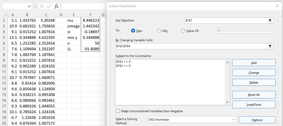
Figure 1 – Using Solver to maximize LL

After clicking on the Solver button, the results shown in Figure 2 appear.

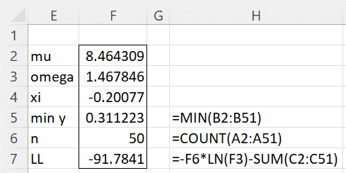
Figure 2 – Maximized LL results

We see that the parameters shown in range F2:F4 of Figure 2 yield a larger value for LL than those calculated by the method of moments, as shown in Figure 1.

Example (Real Statistics approach)

Example 2: Repeat Example 1 using the GEV_FITM and GEV_FIT worksheet functions described in Real Statistics Support for Method of Moments and Real Statistics Support for MLE.

The results are shown in Figure 2. Range J1:N4 contains results for the MLE approach using the array formula =GEV_FIT(A2:A51,TRUE,,,,8.7,1.3,-0.1). Range J6:K9 contains the results using the method of moments via the array formula =GEV_FITM(A2:A51,TRUE,0.05).

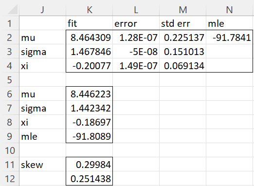
Figure 3 – Maximize LL using GEV_FIT

We used -.1 as the initial guess for the xi parameter in the GEV_FITM formula. We could have used a wide range of initial guesses, but these values need to be less than 1/3. For values of xi > 1/3, the g3 value becomes negative, which introduces problems.

For GEV_FIT, we typically choose initial parameter values close to those produced by GEV_FITM. In fact, if you set the initial guess for sigma to zero, then the method of moment parameter values will be used as the initial values for GEV_FIT by default.

We see that the MLE algorithm converged since the values in range L2:L4 are close to zero. The parameter values and MLE are the same as those shown in Figure 2. The Real Statistics function also returns standard errors for the fit parameters. Thus, we have a 95% confidence interval for mu of

8.464309 ± 1.959964 ⋅ .225137

where 1.959964 = NORM.S.INV(1-.025). Thus, the 95% confidence interval for mu is (8.023, 8.906). The confidence intervals for sigma and xi are calculated in a similar manner.

We also see that the parameter estimates based on the method of moments are the same as those shown in Figure 1 of Method of Moments: GEV Distribution.

Finally, note that the skewness value based on the method of moments is 0.29984 (cell K11), which is, as expected, the same as the sample skewness value, while the skewness value based on the MLE is .251438. These values are calculated using the following worksheet function.

Worksheet Function

Real Statistics Function: The Real Statistics Resource Pack provides the following function.

         GEVSKEW(xi) = the skewness value for the GEV distribution based on the xi value

The mu and sigma values can be obtained using the MEAN_DIST and VAR_DIST functions.

Examples Workbook

Click here to download the Excel workbook with the examples described on this webpage.

References

Martins, E. S., Stedinger, J. R. (2000) Generalized maximum-likelihood generalized extreme-value quantile estimators for hydrologic data
https://repositorio.ufc.br/bitstream/riufc/59412/1/2000_art_esmartins3.pdf

Fawcett, L. (2012) Classical model for extremes
http://www.mas.ncl.ac.uk/~nlf8/teaching/mas8391/background/chapter2.pdf