Basic Concepts
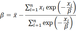
The log-likelihood function for the Gumbel distribution for the sample {x1, …, xn} is
![]()
To estimate the parameters using the MLE method, we need to simultaneously solve the following two equations (proof requires calculus):

Example
Example 1: Every day, the concentration of Zercon ions in the atmosphere was measured, and the maximum such value over the span of 50 days was recorded. The last 15 such measurements are shown in column R of Figure 1. What is the probability that the maximum Zercon measurement over the next 50 days will exceed a dangerous level of 3.5, assuming that these maximum values follow a Gumbel distribution?
The Gumbel distribution was chosen since it captures extreme values as described in Gumbel Distribution.

Figure 1 – Method of Moments
Note that a Zircon ion is completely my invention and doesn’t really exist in nature. In fact, each of the 15 measurements in column R comes from creating 50 random values from a standard normal distribution and selecting the maximum value.
Iterative approach
The approach using the Maximum Likelihood Estimation (MLE) is a bit more complicated and requires 7 or 8 iterations, as shown in columns C through J of Figure 2, using the beta value calculated by the method of moments as the initial guess (cell C2). The beta values, shown in row 2 converge to the value .349323 (cell J2).
We now explain how we obtained the first improved guess for beta of .347061 (cell D2). Since, as we have seen above
we calculate the value shown on the right side of this formula to obtain a new value for beta (actually, we use the average of the old and new values to speed up the convergence).
This is done by inserting the formula =EXP(-$A3/C$2) in cell C3, highlighting the range C3:C17, and pressing Ctrl-D. The new value of beta is now obtained by inserting the following formula in cell C19 (where cell A8 contains the mean of the data elements).
=$A$18-SUMPRODUCT($A3:$A17,C3:C17)/SUM(C3:C17)
and the formula =(C2+C19)/2 in cell D2.
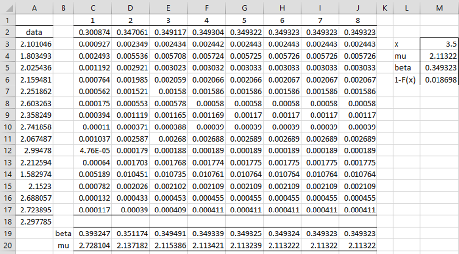
Figure 2 – MLE Method
The rest of the iteration is done by highlighting the range C3:J19 and pressing Ctrl-R and highlighting the range D2:J2 and pressing Ctrl-R. Once the beta value is obtained, the estimate for mu (cell J20) is obtained using the following formula.
=-J19*LN(AVERAGE(J3:J17))
Conclusion
From these parameters, we can calculate the probability that x > 3.5 using the GUMBEL_DIST function to obtain the value of 1.9% (cell M6). Using this approach, we see that the probability of reaching dangerous Zercon levels is almost 2%.
Examples Workbook
Click here to download the Excel workbook with the examples described on this webpage.
References
Wikipedia (2020) Gumbel distribution
https://en.wikipedia.org/wiki/Gumbel_distribution
Hastings, N., Peacock, B. (2011) Statistical distributions. 4th Ed, Wiley
https://www.wiley.com/en-us/Statistical+Distributions%2C+4th+Edition-p-9780470390634
Hi Charles,
Thanks for all you’ve done with using statistics in Excel. It’s a great way to really learn and understand many of the more difficult statistical methods. I may be missing something obvious but isn’t the mean of the Gumbel u + B*.5772? The formula in cell U6 in Fig 1 shows it as u – B*.5772
Hi Bill,
Glad you like Real Statistics.
Yes, mean = mu + b*.5772. Solving for mu yields mu = mean – b*.5772. Mu is not the mean.
Charles
To be more precise on the Gumbel random deviates, perhaps better, create a data set employing U (a random Uniform deviate as supplied by the RAND() function) upon equating to the cumulative distribution function (or CDF) of the Gumbel, and solve for the required Gumbel’s Xi deviate (this is a Monte Carlo simulation method via direct CDF inversion when possible) in terms of U and the provided Gumbel’s parameters.