Basic Concepts
When the chi-square test of independence produces a significant result, indicating that it is unlikely that the two variables are independent, it is often desirable to pinpoint which components of the two variables are responsible for the significant result. This can often be done by using additional chi-square tests of independence based on a subset of the original contingency table.
Example
Example 1: Perform a follow-up analysis for Example 1 of Independence Testing using only the data for Wealthy and Poor people.
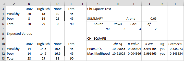
Figure 1 – Post-hoc analysis
We see from Figure 1 that a person’s schooling is not independent of their parents’ wealth even when restricted just to Wealthy vs. Poor parents.
But there are other possibilities: we can compare Wealthy with Middle or Middle with Poor. Similarly, we can compare University with High School or University with None or High School with None (by removing one column instead of one row of the contingency table).
Alternative Tests
There are 3 possible tests where one row is removed and 3 possible tests where one column is removed, for a total of 6 such tests. As described in Multiple Comparisons using Bonferroni Correction, performing multiple follow-up tests introduces familywise error. We can deal with this sort of issue by using a Bonferroni correction. E.g. if we plan to conduct all six of these follow-up tests then we need to use .05/6 = .00833 as the significance level instead of alpha = .05.
If we know in advance of conducting the experiment (and certainly before collecting any data) we know that we only plan to carry out two of these tests, and we specify in advance which two tests we will carry out, then we only need to use a Bonferroni correct of .05/2 = .025.
Thus, if we carried out all six of the post-hoc tests described above, then we would still find that the test in Example 1 is still significant since p-value = .005804 < .008333. In fact, if we carry out all six tests, we will find that the other significant tests are where Wealthy is removed (p-value = .001098) and where High School is removed (p-value = .000402). For this example, the results not have changed if a Bonferroni correction was not made, but this is not necessarily the case in general.
The problem is even more complicated than what we have stated thus far. We can also leave out one row and one column of the contingency table (resulting in a 2 × 2 table such as Wealthy/Poor with University/High School).
Output
There are even more possible post-hoc tests such as Poor/Not Poor with University/No University. Here, we add two columns and/or two rows together. This analysis is shown in Figure 2.

Figure 2 – Another post-hoc analysis
Once again, we get a significant result. Note that the value in cell B4 is equal to the value in B6+B7 from Figure 1 of Independence Testing, the value in cell B5 is equal to the value in cell B8 from that figure, the value in cell C4 is equal to the value C6+C7+D6+D7 from that figure, and the value in cell C5 is equal to the value C8+D8.
Standard Residuals
Another approach to post-hoc testing is to determine which cells are playing the biggest and smallest role in the independence test. This is done by calculating the standard residuals of each cell as follows:
![]()
For samples that are sufficiently large, the standard residuals play the same role as z-scores. Values that are larger in absolute value than NORM.S.INV(1–α/2) are considered to be significant. Thus, for α = .05, cells that have a standard residual whose absolute value is larger than 1.96 can be viewed as significant. For Example 1 of Independence Testing, the standard residuals are as shown in Figure 3.
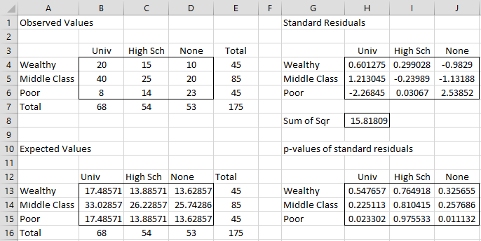
Figure 3 – Standard Residuals
E.g. cell H4 contains the formula =(B4-B13)/SQRT(B13) and cell H13 contains the formula =2*NORM.S.DIST(-ABS(H4), TRUE).
We see that Poor/None and Poor/Univ are significant (for α = .05) since cells J6 and H6 are larger than 1.96 in absolute value (or alternatively cells J16 and H15 are less than .05).
Note too that the sum of squares of the standard residuals is equal to the chi-square test statistic. In Figure 3, we see that cell H8, as calculated by the formula =SUMSQ(H4:J6), contains the same value, 15.81809, as that produced by the formula =CHI_STAT(B4:D6).
Adjusted Residuals
Another approach is to use the adjusted residuals, which are defined as
![]()
where rowp = the row proportion and colp = the column proportion. For Example 1 of Independence Testing
Adjusted residuals give a more accurate picture of the importance of each cell in the contingency table. For Example 1 of Independence Testing, the adjusted residuals are shown in Figure 4.
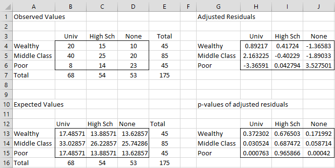
Figure 4 – Adjusted Residuals
Cell H4 contains the formula =(B4-B13)/SQRT(B13*(1-B13/$E13)*(1-B13/B$16)) and cell H13 contains the formula =2*NORM.S.DIST(-ABS(H4), TRUE).
This time, in addition to the significant cells shown in Figure 3, we also see that Middle Class/Univ is significant.
Real Statistics Support
As described in Independence Testing, the Chi-square Test for Independence data analysis tool displays the adjusted residuals.
Click here for additional information about how to conduct post-hoc tests using the Real Statistics Resource Pack.
Examples Workbook
Click here to download the Excel workbook with the examples described on this webpage.
References
Newsom, J. T. (2000) Lecture 13, More on chi-square
http://web.pdx.edu/~newsomj/pa551/lectur13.htm
Agresti, A. (2013) Categorical data analysis, 3rd Ed. Wiley.
https://mybiostats.files.wordpress.com/2015/03/3rd-ed-alan_agresti_categorical_data_analysis.pdf
Naioti, E., Mudrak, E. (2022) Using adjusted standardized residuals for interpreting contingency tables
https://cscu.cornell.edu/wp-content/uploads/conttableresid.pdf