Goodness-of-Fit to a Distribution

Fitting data to a distribution

We can also apply the chi-square goodness of fit test (both the Pearson’s and maximum likelihood versions) to determine whether observed data fit a certain distribution (or curve). For this purpose, we employ the following modified version of Property 1 or 2 of Goodness of Fit.

Property 1: Where there are m unknown parameters in the distribution or curve being fitted, the test statistic in Property 2 of Goodness of Fit has approximately the chi-square distribution χ² (k–m–1).

Thus when fitting data to a Poisson distribution m = 1 (the mean parameter), while if fitting data to a normal distribution m = 2 (the mean and standard deviation parameters).

Goodness-of-fit example

Example 1: A substance is bombarded with radioactive particles for 200 minutes. Between 0 and 7 hits were observed in any one-minute interval, as summarized in columns A and B of the worksheet in Figure 1. Thus for 8 of the one-minute intervals, there were no hits, for 33 of the one-minute intervals, there was 1 hit, etc.

Figure 1 – Example data plus chi-square calculation

We hypothesize that the data follows a Poisson distribution whose mean is the weighted average of the observed number of hits per minute, which we calculate to be 612/200 = 3.06 (cell B14).

H₀: the observed data follows a Poisson distribution

For each row in the table, we next calculate the probability of x (where x = hits per minute) for x = 0 through 7 using the Poisson pdf, i.e. f(x) = POISSON.DIST(x, 3.06, FALSE), and then multiply this probability by 200 to get the expected number of hits per interval assuming the null hypothesis is true (column D). For example, cell D4 contains the worksheet formula =POISSON.DIST(A4,$B$14,FALSE)*B$12.

Analysis

We would like to proceed as in Example 3 of Goodness of Fit, except that this time we can’t use CHISQ.TEST since df ≠ the sample size minus 1. In fact, df = k – m – 1 = 8 – 1 – 1 = 6 since there are 8 intervals (k) and the Poisson distribution has 1 unidentified parameter (m), namely the mean. We, therefore, proceed as in Example 2 of Goodness of Fit, and explicitly calculate the chi-square test statistic (in column F) to be 3.085. We next calculate the following:

p-value = CHISQ.DIST.RT(χ², df) = CHISQ.DIST.RT(3.085,6) = .798 > .05 = α

χ²-crit = CHISQ.INV.RT(α, df) = CHISQ.INV.RT(.05,6) = 12.59 > 3.09 = χ²-obs

Based on either of the above inequalities, we retain the null hypothesis, and so with 95% confidence conclude that the observed data follow a Poisson distribution.

Worksheet Function

Real Statistics Function: The Real Statistics Resource Pack provides the following function to handle analyses such as that used for Example 1:

FIT_TEST(R1, R2, par) = CHISQ.DIST.RT(χ², df) where R1 = the array of observed data, R2 = the array of expected values, par = the number of unknown parameters as in Property 1 (default = 0), and χ² is calculated from R1 and R2 as in Definition 2 with df = the number of elements in R1 (or R2) – par – 1.

For Example 2 of Goodness of Fit, FIT_TEST(B4:G4,B5:G5) = CHISQ.TEST(B4:G4,B5:G5) = .0297 and for Example 1, FIT_TEST(B4:B11,D4:D11,1) = .798.

Observation: See Chi-square Goodness-of-Fit Test and Goodness-of-Fit Analysis Tools for additional information about how to use Real Statistics capabilities to perform a chi-square goodness-of-fit test for specific distributions.

Testing using the index of dispersion

As we saw above, we can use Property 1 to determine whether data follow a Poisson distribution. Note that if we want to test whether data follow a Poisson distribution with a predefined mean then we can use Property 2 of Goodness of Fit instead, and so don’t need to reduce the degrees of freedom of the chi-square test by one.

We can also use the index of dispersion (described at Poisson Distribution) to test whether a data set follows a Poisson distribution. 

Definition 1: The Poisson index of dispersion is defined as

Since the index of dispersion is the variance divided by the mean, the Poisson index of dispersion is simply the index of dispersion multiplied by n−1. The Poisson index of dispersion for the data in R1 can be calculated by the Excel formula =DEVSQ(R1)/AVERAGE(R1).

Property 2: For a sample of sufficiently large size n and mean ≥ 4, the Poisson index of dispersion follows a chi-square distribution with n–1 degrees of freedom.

The estimate is pretty good when the mean ≥ 4 even for values of n as low as 5. Thus the property is especially useful with small samples, where we don’t have sufficient data to use the goodness-of-fit test described previously.

Poisson Index of Dispersion Example

Example 2: Use Property 2 to determine whether the data in range A3:B8 of Figure 2 follows a Poisson distribution.

As we can see from the analysis in Figure 2, we don’t have sufficient reason to reject the null hypothesis that the data follows a Poisson distribution.

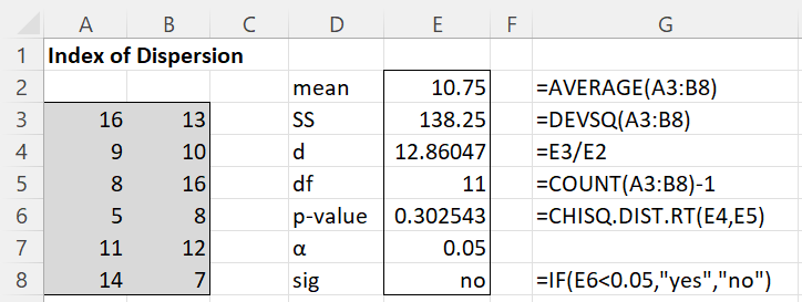
Figure 2 – Testing using Poisson Index of Dispersion

Examples Workbook

Click here to download the Excel workbook with the examples described on this webpage.

References

Zar, J. H. (2010) Biostatistical analysis 5^th Ed. Pearson
https://bayesmath.com/wp-content/uploads/2021/05/Jerrold-H.-Zar-Biostatistical-Analysis-5th-Edition-Prentice-Hall-2009.pdf

Agresti, A. (2013) Categorical data analysis, 3rd Ed. Wiley.
https://mybiostats.files.wordpress.com/2015/03/3rd-ed-alan_agresti_categorical_data_analysis.pdf

Howell, D. C. (2010) Statistical methods for psychology (7^th ed.). Wadsworth, Cengage Learning.
https://labs.la.utexas.edu/gilden/files/2016/05/Statistics-Text.pdf