Statistical Power
We begin by showing how to calculate the power of a one-sample t-test using the approach from Power of a Sample for the normal distribution. In Statistical Power of the t Tests we show another way of computing statistical power using the noncentral t distribution.
Example 1: A university research group wanted to verify the results of a previous study done at another research institution in promoting the production of protective factors for wheat plants by using a combination of chemicals called Formula Y. The previous study reported that the mean concentration of such protective factors after an application of Formula Y was 52. The new study examined 20 wheat plants with the concentration of protective factors shown on the left side of Figure 6. Determine whether the new study is consistent with the previous results. Also, determine the power of the new study.
We begin by exploring the one-tailed test where the null hypothesis is H0: μ ≤ 52; later we will look at the power of the two-tailed test.
The usual one-sample hypothesis testing is shown on the upper right side of Figure 1. We now turn our attention to the power analysis, shown on the lower right side of the figure.
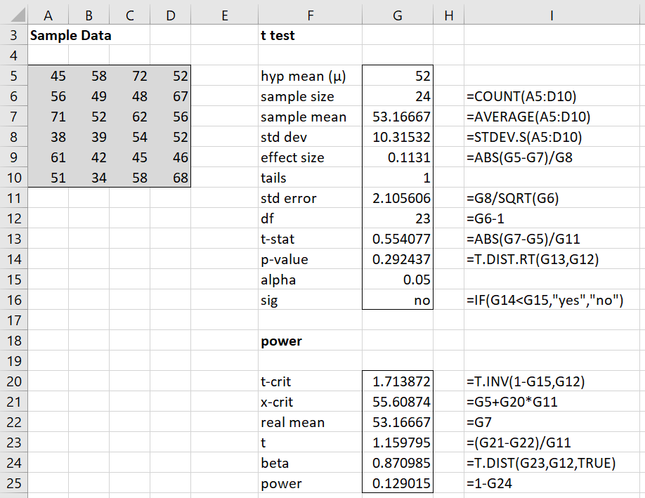
Figure 1 – Calculation of power for a one-tailed test
Let xcrit be the protective factor concentration corresponding to tcrit. Thus,
![]()
and so xcrit = 1.713872 ∙ 2.105606 + 52 = 55.60874. We now assume the real population mean is the sample mean, namely 53.16667. As we saw in Power of a Sample, the situation is illustrated in Figure 2, where the curve on the left represents the t distribution being tested with mean μ0 = 52 and the normal curve on the right represents the distribution with mean μ1 =53.16667.

Figure 2 – Statistical power
When xcrit = 55.60874, the t statistic for the t distribution with mean 53.16667 is
![]()
Thus we have
β = P(t ≤ tcrit | μ = μ1) = T_DIST(1.159795, 23, TRUE) = 0.870985
And so power = 1 – β = .129015.
Note that T_DIST(t, df, TRUE) is equivalent the following formula:
=IF(t >= 0, TDIST(t, df, 1), 1 – TDIST(-t, df, 1))
or T.DIST(t, df, TRUE) in releases of Excel starting with Excel 2010.
The specific test that was conducted did not reject the null hypothesis, but we also see that such a test would only have found a very small effect of size .1136 (cell G9 of Figure 1) 12.9% of the time, which is quite poor. Shortly we will consider some of the ways of increasing power to more acceptable levels.
For each value of μ1 ≥ 52 we can repeat the above calculations to obtain a value of power. From these, we obtain the power plot shown in Figure 3.

Figure 3 – Power curve for Example 1
Observation: We are about to conduct a series of what-if analyses. We will use the format shown in Figure 4 for each of these analyses, where the figure repeats the power calculation for Example 1.
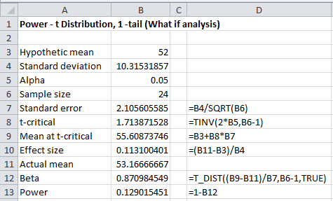
Figure 4 – What if analysis (based on given mean)
Example 2: For the data in Example 1, answer the following questions:
- What is the power of the test for detecting a standardized effect of size .4?
- What effect size (and mean) can be detected with power .80?
- What sample size is required to detect an effect of size .2 with power .80?
a) As described above, we use the following measure of effect size:
![]()
Thus μ1 = 752 + (.4)(10.31532) = 56.12612743. As in Example 1, we can then calculate the power of the test to be 59.6% as described in Figure 5:
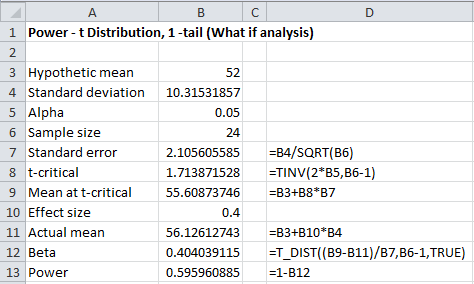
Figure 5 – Calculating the power of a one-tailed t-test
b) We use Excel’s Goal Seek capability to answer the second question. Using the worksheet in Figure 5, we now select Data > Data Tools | What-If Analysis. In the dialog box that appears, enter the following values:

Figure 6 – Determine effect size required to obtain power of .80
We are requesting that Excel find the value of cell B10 (the effect size) that produces a value of .8 for cell B13 (the power). Here the first entry must point to a cell that contains a formula. The second entry must be a value and the third entry must point to a cell that contains a value (possibly blank) and not a formula. After clicking on the OK button, a Goal Seek Status dialog box appears, and the worksheet from Figure 5 changes to that in Figure 7.
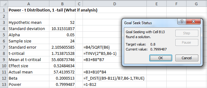
Figure 7 – Output from Goal Seek to determine effect size
Note that the values of a number of cells have changed to reflect the value necessary to obtain power of .80. In particular, we see that the Effect size (cell B10) contains the value 0.52484634. You must click on the OK button to lock in these new values (or Cancel to return to the original worksheet).
c) We again use Excel’s Goal Seek capability to answer the third question. Using the worksheet in Figure 4 (making sure that the effect size in cell B10 is set to .2), we now enter the following values in the dialog box that appears (see Figure 8):
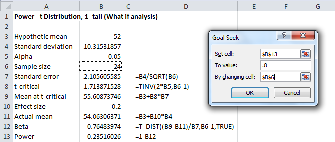
Figure 8 – Goal Seek dialog box to obtain sample size
After clicking on OK, the worksheet changes to that in Figure 9.
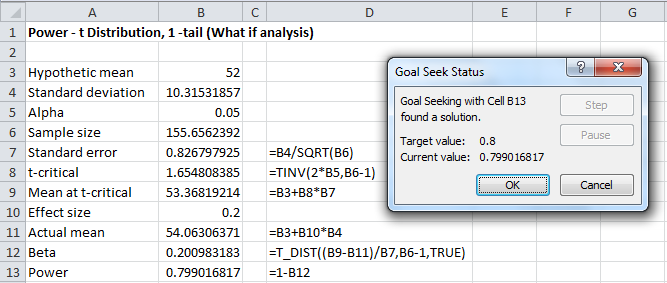
Figure 9 – Output from Goal Seek to determine sample size
In particular, note that the sample size value in cell B6 changes to 155.6562392. Thus the required sample size is 156 (rounding up to the nearest integer).
Example 3: Repeat Example 1 using a two-tailed test, i.e. where the null hypothesis is H0: μ = 52.
We note that the picture shown in Figure 2 changes to that shown in Figure 10.
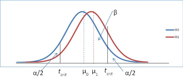
Figure 10 – Power for a two-tailed test
The blue curve represents the t distribution assuming that the null hypothesis is true (where μ0 = 52 for our example). The two critical regions (left and right) are determined by the left and right critical values tcrit. The red curve represents the t distribution assuming that the null hypothesis is false (i.e. the alternative hypothesis is true). For our example we assume that the real population mean is given by the sample mean, i.e. μ1 = 53.16667. The value of beta is therefore the region bounded by the red curve, the x-axis and the line y = t-crit and y = t+crit. Power is then 1−β.
The analysis for Example 3 is shown in Figure 11.
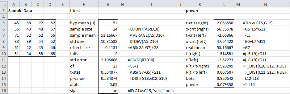
Figure 11 – Calculation of power for a two-tailed t-test
The power for the two-tailed test (cell L15) is 7.9%, which as expected is lower than the power for the one-tailed test.
Charles,
In Example 1, the previous study reports the mean of their results (52) but not the standard deviation or sample size. If these are known, would it be better to calculate the t-test effect size using the pooled std dev instead of the new std dev (10.31532), as shown in Fig. 1?
Thanks.
Hello Dave,
Yes, that might be preferable since you would include all available information. I need to study this further to say for sure.
Charles