Basic Concepts
We now show how to create a nonlinear exponential regression model using Newton’s Method.
Property 1: Given samples {x1, …, xn} and {y1, …, yn} and let ŷ = αeβx, then the value of α and β that minimize 
![]()
![]()
Proof: For a proof using calculus, click here
Property 2: Under the same assumptions as Property 1, given initial guesses α0 and β0 for α and β, let F = [f g]T where f and g are as in Property 1 and

Now define the 2 × 1 column vectors Bn and the 2 × 2 matrices Jn recursively as follows
![]()
![]()
![]()
Then provided α0 and β0 are sufficiently close to the coefficient values that minimize the sum of the deviations squared, then Bn converges to such coefficient values.
Proof: For a proof using calculus, click here
Property 3: The approximate covariance matrix for the coefficients vector is given by
![]()
where![]()
Example
Example 1: We now show how to calculate the value of the α and β coefficients for the exponential regression model for the data in Example 1 of Exponential Regression using a Linear Model or Exponential Regression using Solver (repeated in range A3:B14 of Figure 0), this time using Newton’s Method (i.e. Property 2).

Figure 0 – Data for Example 1
The first 5 iterations of Newton’s method are shown in Figure 1. As you can see the coefficients calculated in step 5 (range B31:B32) are the same as those in step 4 (range B28:B29) and so convergence is reached after 5 steps, with values α = 12.50475 and β = .016854.
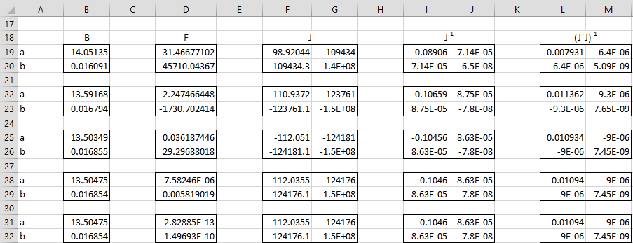
Figure 1 – Exponential Regression using Newton’s Method
In Figure 2 we show key formulas used in Figure 1 based on Property 1 and 2 and referencing the input X data in range A4:A14 and Y data in range B4:B14 from Figure 1 of Exponential Regression using Solver.
| Item | Cells | Formula |
| B0 | B19:B20 | use values from Excel exponential regression |
| F0 | D19 | =SUMPRODUCT(SUMPRODUCT($B$4:$B$14-B19*EXP(B20*$A$4:$A$14),EXP(B20*$A$4:$A$14))) |
| D20 | =B19*SUMPRODUCT(SUMPRODUCT($B$4:$B$14-B19*EXP(B20*$A$4:$A$14),EXP(B20*$A$4:$A$14),$A$4:$A$14)) | |
| J0 | F19 | =-SUMPRODUCT(EXP(2*B20*$A$4:$A$14)) |
| G19 | =SUMPRODUCT(SUMPRODUCT($B$4:$B$14-2*B19*EXP(B20*$A$4:$A$14),EXP(B20*$A$4:$A$14),$A$4:$A$14)) | |
| F20 | =G19 | |
| G20 | =B19*SUMPRODUCT(SUMPRODUCT($B$4:$B$14-2*B19*EXP(B20*$A$4:$A$14),EXP(B20*$A$4:$A$14),$A$4:$A$14^2)) | |
| J0-1 | I19:J20 | =MINVERSE(F19:G20) |
| B1 | B22:B23 | =B19:B20-MMULT(I19:J20,D19:D20) |
Figure 2 – Formulas from Figure 1
We can now create the regression analysis as shown in Figure 3.

Figure 3 – Exponential Regression results using Newton’s Method
Figure 4 displays key formulas from Figure 3, referencing the cells in Figure 1.
| Item | Cells | Formula |
| α coefficient | P25 | =B31 |
| β coefficient | P26 | =B32 |
| α s.e. | Q25 | =SQRT(L31*R21) |
| β s.e. | Q26 | =SQRT(M32*R21) |
| SSE | Q21 | =SUMPRODUCT((B4:B14-B31*EXP(B32*A4:A14))^2) |
| MSE | R21 | =Q21/P21 |
Figure 4 – Formulas from Figure 3
Alternative Approach
The following is an alternative approach for finding the regression coefficients α and β. By Property 1
![]()
Thus, if α ≠ 0 we can solve for α to get
![]()
Thus, we can replace the original two equations in two unknowns by the following equation in one unknown:
![]()
This can be solved iteratively using Newton’s Method in one variable, as described in Newton’s Method.
Observation: There is another algorithm that is commonly used to find the regression coefficients called the Levenberg-Marquardt algorithm, which combines the advantages of Newton’s Method with those of the algorithm used by Solver. We won’t consider this algorithm further here.
Examples Workbook
Click here to download the Excel workbook with the examples described on this webpage.
Link
References
Foth, R. (2024) Modeling exponential relationships with regression
https://pimaopen.pressbooks.pub/topicsinmathematics/chapter/5-4-modeling-exponential-relationships-with-regression
Abramson, J. (2024) Exponential and logarithmic regressions
https://math.libretexts.org/Workbench/1250_Draft_3/06%3A_Exponential_and_Logarithmic_Functions/6.09%3A_Exponential_and_Logarithmic_Regressions
Libre Texts (2024) Nonlinear regression
https://math.libretexts.org/Workbench/Numerical_Methods_with_Applications_(Kaw)/6%3A_Regression/6.04%3A_Nonlinear_Regression
Geeks for Geeks (2024) Non-linear regression with examples
https://www.geeksforgeeks.org/non-linear-regression-examples-ml/