Principal Component Analysis

Principal component analysis is a statistical technique that is used to analyze the interrelationships among a large number of variables and to explain these variables in terms of a smaller number of variables, called principal components, with a minimum loss of information.

Definition 1: Let X = [x_i] be any k × 1 random vector. We now define a k × 1 vector Y = [y_i], where for each i the ith principal component of X is

for some regression coefficients β_ij. Since each y_iis a linear combination of the x_j, Y is a random vector.

Now define the k × k coefficient matrix β = [β_ij] whose rows are the 1 × k vectors $\beta^T X$ = [β_ij]. Thus,

y_i = $\beta_i^T X$ Y = $\beta^T X$

For reasons that will be become apparent shortly, we choose to view the rows of β as column vectors β_i, and so the rows themselves are the transpose $\beta_i^T X$ .

Observation: Let Σ = [σ_ij] be the k × k population covariance matrix for X. Then the covariance matrix for Y is given by

Σ_Y = β^TΣ β

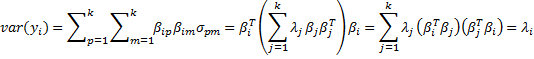
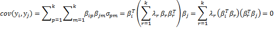
i.e. population variances and covariances of the y_i are given by

Observation: Our objective is to choose values for the regression coefficients β_ij so as to maximize var(y_i) subject to the constraint that cov(y_i, y_j) = 0 for all i ≠ j. We find such coefficients β_ij using the Spectral Decomposition Theorem (Theorem 1 of Linear Algebra Background). Since the covariance matrix is symmetric, by Theorem 1 of Symmetric Matrices, it follows that

Σ = β D β^T

where β is a k × k matrix whose columns are unit eigenvectors β₁, …, β_k corresponding to the eigenvalues λ₁, …, λ_k of Σ and D is the k × k diagonal matrix whose main diagonal consists of λ₁, …, λ_k. Alternatively, the spectral theorem can be expressed as

Property 1: If λ₁ ≥ … ≥ λ_k are the eigenvalues of Σ with corresponding unit eigenvectors β₁, …, β_k, then

and furthermore, for all i and j ≠ i

var(y_i) = λ_i cov(y_i, y_j) = 0

Proof: The first statement results from Theorem 1 Symmetric Matrices as explained above. Since the column vectors β_j are orthonormal, β_i · β_j = $\beta_i^T \beta_j$ = 0 if j ≠ i and $\beta_i^T \beta_j$ = 1 if j = i. Thus

Property 2:

Proof: By definition of the covariance matrix, the main diagonal of Σ contains the values $\sigma_1^2$ , …, $\sigma_k^2$ , and so trace(Σ) = $\sum_{i=1}^k \sigma_i^2$ . But by Property 1 of Eigenvalues and Eigenvectors, trace(Σ) = $\sum_{i=1}^k \lambda_i$ .

Observation: Thus the total variance $\sum_{i=1}^k \sigma_i^2$ for X can be expressed as trace(Σ) = $\sum_{i=1}^k \lambda_i$ , but by Property 1, this is also the total variance for Y.

Thus the portion of the total variance (of X or Y) explained by the ith principal component y_i is λ_i/ $\sum_{i=1}^k \lambda_i$ . Assuming that λ₁ ≥ … ≥ λ_k the portion of the total variance explained by the first m principal components is therefore $\sum_{i=1}^m \lambda_i$ / $\sum_{i=1}^k \lambda_i$ .

Our goal is to find a reduced number of principal components that can explain most of the total variance, i.e. we seek a value of m that is as low as possible but such that the ratio $\sum_{i=1}^m \lambda_i$ / $\sum_{i=1}^k \lambda_i$ is close to 1.

Observation: Since the population covariance Σ is unknown, we will use the sample covariance matrix S as an estimate and proceed as above using S in place of Σ. Recall that S is given by the formula:

where we now consider X = [x_ij] to be a k × n matrix such that for each i, {x_ij: 1 ≤ j ≤ n} is a random sample for random variable x_i. Since the sample covariance matrix is symmetric, there is a similar spectral decomposition

where the B_j = [b_ij] are the unit eigenvectors of S corresponding to the eigenvalues λ_j of S (actually this is a bit of an abuse of notation since these λ_j are not the same as the eigenvalues of Σ).

We now use b_ij as the regression coefficients and so have

and as above, for all i and j ≠ i

var(y_i) = λ_i cov(y_i, y_j) = 0

As before, assuming that λ₁ ≥ … ≥ λ_k, we want to find a value of m so that $\sum_{i=1}^m \lambda_i$ explains as much of the total variance as possible. In this way we reduce the number of principal components needed to explain most of the variance.

Example 1: The school system of a major city wanted to determine the characteristics of a great teacher, and so they asked 120 students to rate the importance of each of the following 9 criteria using a Likert scale of 1 to 10 with 10 representing that a particular characteristic is extremely important and 1 representing that the characteristic is not important.

Setting high expectations for the students
Entertaining
Able to communicate effectively
Having expertise in their subject
Able to motivate
Caring
Charismatic
Having a passion for teaching
Friendly and easy-going

Figure 1 shows the scores from the first 10 students in the sample and Figure 2 shows some descriptive statistics about the entire 120 person sample.

Figure 1 – Teacher evaluation scores

Descriptive statistics teacher evaluations

Figure 2 – Descriptive statistics for teacher evaluations

The sample covariance matrix S is shown in Figure 3 and can be calculated directly as

=MMULT(TRANSPOSE(B4:J123-B126:J126),B4:J123-B126;J126)/(COUNT(B4:B123)-1)

Here B4:J123 is the range containing all the evaluation scores and B126:J126 is the range containing the means for each criterion. Alternatively, we can simply use the Real Statistics formula COV(B4:J123) to produce the same result.

Covariance matrix teacher evealuation

Figure 3 – Covariance Matrix

In practice, we usually prefer to standardize the sample scores. This will make the weights of the nine criteria equal. This is equivalent to using the correlation matrix. Let R = [r_ij] where r_ij is the correlation between x_i and x_j, i.e.

The sample correlation matrix R is shown in Figure 4 and can be calculated directly as

=MMULT(TRANSPOSE((B4:J123-B126:J126)/B127:J127),(B4:J123-B126:J126)/B127:J127)/(COUNT(B4:B123)-1)

Here B127:J127 is the range containing the standard deviations for each criterion. Alternatively, we can simply use the Real Statistics function CORR(B4:J123) to produce the same result.

Correlation matrix teacher evaluations

Figure 4 – Correlation Matrix

Note that all the values on the main diagonal are 1, as we would expect since the variances have been standardized. We next calculate the eigenvalues for the correlation matrix using the Real Statistics eigVECTSym(M4:U12) formula, as described in Linear Algebra Background. The result appears in range M18:U27 of Figure 5.

Eigenvalues eigenvectors correlation matrix

Figure 5 – Eigenvalues and eigenvectors of the correlation matrix

The first row in Figure 5 contains the eigenvalues for the correlation matrix in Figure 4. Below each eigenvalue is a corresponding unit eigenvector. E.g. the largest eigenvalue is λ₁ = 2.880437. Corresponding to this eigenvalue is the 9 × 1 column eigenvector B₁ whose elements are 0.108673, -0.41156, etc.

As we described above, coefficients of the eigenvectors serve as the regression coefficients of the 9 principal components. For example, the first principal component can be expressed by

This can also be expressed as

Thus for any set of scores (for the x_j) you can calculate each of the corresponding principal components. Keep in mind that you need to standardize the values of the x_j first since this is how the correlation matrix was obtained. For the first sample (row 4 of Figure 1), we can calculate the nine principal components using the matrix equation Y = BX′ as shown in Figure 6.

Figure 6 – Calculation of PC1 for first sample

Here B (range AI61:AQ69) is the set of eigenvectors from Figure 5, X (range AS61:AS69) is simply the transpose of row 4 from Figure 1, X′ (range AU61:AU69) standardizes the scores in X (e.g. cell AU61 contains the formula =STANDARDIZE(AS61, B126, B127), referring to Figure 2) and Y (range AW61:AW69) is calculated by the formula

=MMULT(TRANSPOSE(AI61:AQ69),AU61:AU69)

Thus the principal component values corresponding to the first sample are 0.782502 (PC1), -1.9758 (PC2), etc.

As observed previously, the total variance for the nine random variables is 9 (since the variance was standardized to 1 in the correlation matrix), which is, as expected, equal to the sum of the nine eigenvalues listed in Figure 5. In fact, in Figure 7 we list the eigenvalues in decreasing order and show the percentage of the total variance accounted for by that eigenvalue.

Figure 7 – Variance accounted for by each eigenvalue

The values in column M are simply the eigenvalues listed in the first row of Figure 5, with cell M41 containing the formula =SUM(M32:M40) and producing the value 9 as expected. Each cell in column N contains the percentage of the variance accounted for by the corresponding eigenvalue. E.g. cell N32 contains the formula =M32/M41, and so we see that 32% of the total variance is accounted for by the largest eigenvalue. Column O simply contains the cumulative weights, and so we see that the first four eigenvalues account for 72.3% of the variance.

Using Excel’s charting capability, we can plot the values in column N of Figure 7 to obtain a graphical representation, called a scree plot.

Figure 8 – Scree Plot

We decide to retain the first four eigenvalues, which explain 72.3% of the variance. In section Basic Concepts of Factor Analysis we will explain in more detail how to determine how many eigenvalues to retain. The portion of Figure 5 that refers to these eigenvalues is shown in Figure 9. Since all but the Expect value for PC1 is negative, we first decide to negate all the values. This is not a problem since the negative of a unit eigenvector is also a unit eigenvector.

Figure 9 – Principal component coefficients (Reduced Model)

Those values that are sufficiently large, i.e. the values that show a high correlation between the principal components and the (standardized) original variables, are highlighted. We use a threshold of ±0.4 for this purpose.

This is done by highlighting the range R32:U40 and selecting Home > Styles|Conditional Formatting and then choosing Highlight Cell Rules > Greater Than and inserting the value .4 and then selecting Home > Styles|Conditional Formatting and then choosing Highlight Cell Rules > Less Than and inserting the value -.4.

Note that Entertainment, Communications, Charisma and Passion are highly correlated with PC1, Motivation and Caring are highly correlated with PC3 and Expertise is highly correlated with PC4. Also, Expectation is highly positively correlated with PC2 while Friendly is negatively correlated with PC2.

Ideally, we would like to see that each variable is highly correlated with only one principal component. As we can see from Figure 9, this is the case in our example. Usually, this is not the case, however, and we will show what to do about this in the Basic Concepts of Factor Analysis when we discuss rotation in Factor Analysis.

In our analysis, we retain 4 of the 9 principal factors. As noted previously, each of the principal components can be calculated by

i.e. Y= B^TX′, where Y is a k × 1 vector of principal components, B is a k x k matrix (whose columns are the unit eigenvectors) and X′ is a k × 1 vector of the standardized scores for the original variables.

If we retain only m principal components, then Y = B^TX where Y is an m × 1 vector, B is a k × m matrix (consisting of the m unit eigenvectors corresponding to the m largest eigenvalues) and X′ is the k × 1 vector of standardized scores as before. The interesting thing is that if Y is known we can calculate estimates for standardized values for X using the fact that X′ = BB^TX’ = B(B^TX′) = BY (since B is an orthogonal matrix, and so, BB^T = I). From X′ it is then easy to calculate X.

Figure 10 – Estimate of original scores using reduced model

In Figure 10 we show how this is done using the four principal components that we calculated from the first sample in Figure 6. B (range AN74;AQ82) is the reduced set of coefficients (Figure 9), Y (range AS74:AS77) are the principal components as calculated in Figure 6, X′ are the estimated standardized values for the first sample (range AU74:AU82) using the formula =MMULT(AN74:AQ82,AS74:AS77) and finally, X are the estimated scores in the first sample (range AW74:AW82) using the formula =AU74:AU82*TRANSPOSE(B127:J127)+TRANSPOSE(B126:J126).

As you can see the values for X in Figure 10 are similar, but not exactly the same as the values for X in Figure 6, demonstrating both the effectiveness as well as the limitations of the reduced principal component model (at least for this sample data).

229 thoughts on “Principal Component Analysis”

Parth

January 20, 2017 at 12:32 pm

Dear Charles
I am not able to understand how we can calculate the Eigenvalue and eigenvector from the covariance matrix. could you please explain me by giving some example.
thanking you
Reply
- Charles
  
  January 20, 2017 at 1:40 pm
  
  Parth,
  It is calculated automatically for you when you use the eVECTORS function or the Factor Analysis data analysis tool.
  If you want to do this manually, then see the following webpages:
  https://real-statistics.com/linear-algebra-matrix-topics/eigenvalues-eigenvectors/
  https://real-statistics.com/linear-algebra-matrix-topics/qr-factorization/
  Charles
  Reply
Sana

December 24, 2016 at 6:22 pm

Just wanted to know, Is it possible somehow to get back co-orelation matrix from eigenvalue and Eigen vector matrix? Futher, can correlation be transformed back to original matix?
Reply
- Charles
  
  December 26, 2016 at 9:26 pm
  
  Sana,
  
  A correlation matrix cannot be transformed back to the original matrix. This fails even for a 1 x 1 correlation matrix, i.e. the correlation between any two variables. Suppose I have two samples and compute the correlation between them. Now suppose I take any linear transformation of one or both of these samples (e.g. I double all the elements in the first sample and add one to all the elements in the second sample. The correlation between these new samples will be the same as the correlation between the original samples.
  
  Regarding your other question, not all eigenvalues can be obtained from some correlation matrix. So we need to ask the related question. If I have a collection of eigenvalues and eigenvectors for some correlation matrix, is it possible that these are also the eigenvalues and eigenvectors for some other correlation matrix? I don’t immediately know the answer to this question.
  
  Charles
  Reply
Ray Rui

December 21, 2016 at 6:12 pm

Hi Charles,
Thank you very much for sharing. I am just studying PCI. I downloaded your excel and read your text. It is very helpful. My question how I can weight for each original variables based on PCA. In your excel, I did not see weight based on PCA for each original variables, e.g. weight for expect, weight for communication variable. Is possible you can update excel or provide some suggestion how to get weight for each original variables from your existing excel example. Thanks.

Ray Rui
Reply
- Charles
  
  January 2, 2017 at 11:39 am
  
  Ray,
  I think you are looking for the factor scores. Please see the following webpage:
  Factor Scores
  Charles
  Reply
MSIS

November 14, 2016 at 1:07 am

Hi Charles,
Thanks for a clear explanation.
Let me see if I my understanding is correct:

1) The covariance matrix E is symmetric, so that it can be diagonalized
as E=ADA^T

Where D_ij is the diagonal matrix with d_ii eigenvalues; A_ik is the matrix where
a_ij is the eigenvector associated with eigenvalue d_ii

2) We can change the basis representing E so that, in this new basis, Cov(x_i,x_j)=0
and Var(x_i)=d_ii

3) This is where I am a bit confused:
The components in PCA are then just the eigenvectors in this new basis satisfying the properties in 2.

Am I close?
Thanks.
Reply
- Charles
  
  November 29, 2016 at 11:07 am
  
  Although I am tempted to wade into the details of your interesting question, I am afraid that I really don’t have the time at present to do this. I am busy trying to complete the writing of a book that is long overdue.
  Charles
  Reply
Prashant Dhamale

October 3, 2016 at 6:57 am

Dear Charles,
Your Example is very good but it has one very basic mistake.
The example you have considered is of ordinal data and Pearson’s correlation coefficient is used for cardinal data.
So i guess you have to use Spearman’s rank correlation to find out the correlation matrix.
Prashant
Reply
- Charles
  
  October 4, 2016 at 9:40 am
  
  Prashant,
  It is common to treat Likert data as interval data. Generally, the larger the range of values, the more reasonable this assumption is. With a range from 1 to 10, I don’t see too much problem.
  Charles
  Reply
David

September 28, 2016 at 12:47 pm

Hi Charles,

Spotted this little typo:
=MMULT(TRANSPOSE(B4:J123-B126:J126),B4:J123-B126;J126)/(COUNT(B4:B123)-1)

Should be
=MMULT(TRANSPOSE(B4:J123-B126:J126),B4:J123-B126:J126)/(COUNT(B4:B123)-1)

>> B126:J126 instead of B126;J126

Regards
Reply
- Charles
  
  September 29, 2016 at 10:40 am
  
  David,
  Thanks for catching this hard-to-spot typo. I had to stare at the formula a couple of times before I found the error. I really appreciate your help in making the website better.
  Charles
  Reply
Michael

June 23, 2016 at 4:41 am

Greetings,

Your example is very helpful. I am curious how this might be applied to the development of indexes for an industry when the most precise data might be time-series NAIC (or SIC) codes from the Census Bureau since this significantly reduces the number of observations.

Any help you could provide would be very much appreciated.

Best wishes,
Michael
Reply
- Charles
  
  June 23, 2016 at 5:56 am
  
  Michael,
  Perhaps because I am not familiar with the NAIC and SIC codes, I don’t exactly understand your question. Can you please provide some background?
  Charles
  Reply
  - Michael
    
    June 23, 2016 at 6:13 pm
    
    Hi Charles,
    
    NAIC’s are the North American Industry Classification system, while SIC’s are the Standard Industry Classification system. These are coding systems used to classify industries such as debt collection, telecommunications, law firms, etc. and correspond with a business’s tax filing code. I hope this helps.
    
    Best wishes,
    Michael
    Reply
    - Charles
      
      June 24, 2016 at 6:18 am
      
      Michael,
      Thanks for explaining this, but I still don’t understand what it is you are looking for from me. I don’t have time to investigate NAIC and SIC to try to figure out how to develop indexes for an industry.
      Charles
      Reply
      - Michael
        
        June 29, 2016 at 2:01 pm
        
        Charles,
        
        Perhaps my reference to NAIC and SIC codes as a frame of reference confused the question. I was only referencing these coding systems since they show aggregate time-series data for numerous industries.
        
        Your above example appears to show a snapshot in time, while I would like to know how PCA would be applied to the development of an index with time-series data.
        
        Once again, sorry for the confusion. I hope this better clarifies my question.
        
        Best wishes,
        Michael
      - Charles
        
        June 30, 2016 at 11:53 am
        
        Sorry Michael, but I just have anything to add to what I said earlier.
        Charles
      - Michael
        
        June 30, 2016 at 1:37 pm
        
        Charles,
        
        Okay, I didn’t think asking about the application of time-series data to PCA was an unreasonable question. Thank you for trying to help.
        
        Best,
        Michael
steve

June 1, 2016 at 5:37 pm

You example is fantastic, thank you

How would these values be used in a regression model? Assuming I want to find a forecast for n and have 9 variables above.
Reply
- Charles
  
  June 1, 2016 at 6:53 pm
  
  Steve,
  Sorry, but I don’t understand your question.
  Charles
  Reply
  - steve
    
    June 1, 2016 at 7:21 pm
    
    Thanks for the prompt reply 🙂
    
    We have produced a model that has reduced our input variables. Can we use this to estimate a given variable not included? Or are we just evaluating the relationships between our input variable (i.e. we can’t predict values from our output).
    
    Thanks again
    Reply
    - steve
      
      June 1, 2016 at 7:58 pm
      
      I guess I am asking if I can use the output from the PCA model in a regression model
      Reply
      - Charles
        
        June 1, 2016 at 9:39 pm
        
        Steve,
        You can map the original data into the factors using the factor scores and then use the use this as input to the regression. See the following webpage for more information.
        https://real-statistics.com/multivariate-statistics/factor-analysis/factor-scores/
        Charles
    - Charles
      
      June 1, 2016 at 9:40 pm
      
      Steve,
      You can use the factor scores, as described in the other response I am providing to you.
      Charles
      Reply
      - steve
        
        June 2, 2016 at 9:30 am
        
        That’s brilliant – I have worked through those examples
        
        Once I have the factor scores the next step is to regress them against the dependent variable, is that correct?
      - Charles
        
        June 2, 2016 at 10:35 am
        
        Yes
Juan Perez

April 26, 2016 at 8:29 pm

Hi Charles, thank you for the explanation.

However, I’m wondering if you could publish all data of the example to try to reproduce your analysis, and then I will feel confidence to do my own. Thank you again!
Reply
- Charles
  
  April 26, 2016 at 10:43 pm
  
  Juan,
  This info is already available. See
  Examples Workbooks
  Charles
  Reply
  - alba~math
    
    May 2, 2017 at 5:21 am
    
    I guess you are talking about the file Real-Statistics-Multivariate-Examples.xlsx Could you please tell which sheet is used in the example of this blogpost.
    Reply
    - Charles
      
      May 2, 2017 at 9:08 am
      
      Yes, it is in that file. You will find it in Principal Component Analysis sheet (in the Factor Analysis group of sheets)
      Charles
      Reply
Jesper Rindboel

April 20, 2016 at 4:57 pm

Dear Charles,
Thank you very much for your tools, they have made my (work)life much easier.

What would be the significance of calculating the eigenvalues of the covariance matrix instead of standardizing the numbers twice (before and after) to work with the correlation matrix?

Regards,
Jesper
Reply
- Charles
  
  April 21, 2016 at 9:57 am
  
  Jesper,
  Glad to see that the tools have been helpful.
  I don’t know what happens if you use the alternative approach that you are describing.
  Charles
  Reply
Muhamamd ( Mu Mu)

April 19, 2016 at 12:20 pm

i am working on Oil Supply Risk assessment.I have 5 Indicators and further 11 subindicators .I want to assingn weights by PCA.can any one help to make me clear how to use PCA with example .I ll be thankful to you. plz send me at mosikhann@yahoo.com Thanks
Muhammad
Reply
- Charles
  
  April 19, 2016 at 2:26 pm
  
  The referenced webpage describes how to do this in general. You haven’t supplied enough information for me to be able to guide you further.
  Charles
  Reply
MGL

April 14, 2016 at 12:34 am

Hi Charles,

I’m going to reference the Excel Spreadsheet File(s) that are provided as examples in this post. I have a few questions.

Real-Statistics-Multivariate-Examples.xls
Tab: PCA

I understand all of the math that is going on after slogging through where the numbers come from. However, in the Excel Sheet that I referenced above, I noticed something strange:

This has to do with the Reduced Model Cells, that have to with Matrix B (AN74:AQ82), Vector Y (AS74:AS77), Vector X’ (AU74:AU82) and Vector X(AW74:AW82)

The Question in particular has to do with the calculation for Vector X, which the formula in Excel is:

AU74:AU82*TRANSPOSE(B127:J127)+TRANSPOSE(B126:J126)

But as I parcel it out, there’s some strange things going on.

If I parcel out TRANSPOSE(B127:J127)+TRANSPOSE(B126:J126), that’s basically an addition of two vectors, the Mean and the Standard Deviation for the nine variables, for which I get values of:

4.974544736
8.736692957
5.099293202
4.397380333
7.664479602
7.377230536
7.431224993
5.677330181
7.888403337

So I put these values into a separate set of cells, let’s just say:

AY74:AY82

But when I do the math of:
AU74:AU82*AY74:AY82

I get:

-4.898239264
-0.660121779
-6.197503264
2.422801034
-2.007222372
-2.098727253
-6.777166555
-1.530919504
11.13149207

These numbers are a lot different than the calculation for the X Vector which is:

2.461544584
8.123596964
1.445506515
3.942037365
6.457931704
5.618899676
2.480028027
4.468199567
8.130308341

So my question is: what is going on here? This may seem like a stupid question, but I am curious as to the calculation that is going on behind the scenes, as it were.

Thanks in advance.
Reply
- MGL
  
  April 14, 2016 at 12:55 am
  
  Oh, nevermind, order of operations. Silly me.
  Reply
Thanh Thao

April 12, 2016 at 10:57 am

Dear Charles,

I dont understand that why dose the eigenvector 1 change the sign between figure 5 and figure 9 ?
in figure 5: 0.108673 in figure 9: -0.108673
-0.41156 0.411555
-0.44432 0.44432
… …
Reply
- Charles
  
  April 12, 2016 at 12:54 pm
  
  If X is a unity eigenvector corresponding to eigenvalue c, then so is -X. I simply changed the sign of all the elements in that eigenvector to keep as many positive values as possible. You should get equivalent values even if you don’t do this.
  Charles
  Reply
Sebastián García

March 30, 2016 at 4:07 pm

How can determine the weight of the variable using Factor Analysis?
Reply
- Charles
  
  March 30, 2016 at 6:13 pm
  
  If you mean loadings, then yes.
  Charles
  Reply
Ahmed

March 27, 2016 at 10:59 pm

very nice explain
kindly Dr. Charles can you attach all data of any example which you explain
i need all data and i will try solve it by any other statistical software like SPSS
Reply
- Charles
  
  March 28, 2016 at 7:39 am
  
  Ahmed,
  You can download all the data from the examples by going to
  Examples Workbooks
  Charles
  Reply
Pingback: Factor Analysis Marketing Example - Marketing on Data
Pingback: Factor Analysis in Marketing - Marketing on Data
Sam Preston

February 3, 2016 at 12:54 pm

Hi Charles,

I commented yesterday on another page having used the Varimax function to give me 10 out of 11 original variables highly correlated with one principal component.

I went on to calculated new X values as shown in Figure 10. I apologise if this is a stupid question (I am new to statistics), but what is the next step? Should the principal components (Y column) be recalculated using the new set of X values?

Thanks again,

Sam
Reply
Rich

January 8, 2016 at 1:36 pm

Happy New Year, Charles

I’m trying to understand more about PCA from your website and using your add-in.

Do you have a posting or discussion that addresses Principal Components Regression in general, and more specifically, using your suite of tools?

Thanks, Rich
Reply
- Charles
  
  January 16, 2016 at 2:44 pm
  
  Rich,
  Happy New Year to you too.
  PCA is usually viewed as a special case of factor analysis. This is explained in detail throughout the Factor Analysis webpages. See Factor Analysis for links to all these pages.
  The Real Statistics tools are described on the webpage Real Statistics Support for Factor Analysis.
  Charles
  Reply
Boro Dega

October 27, 2015 at 2:48 pm

I always see that when plotting the PC’s against each other it is always PC1 against PC2, PC2 against PC3 and so forth…my question is what will be the incentive of plotting PC1 against PC2, PC1 against PC3 so forth..why would I do that and if I do it would that be wrong?
Reply
- Charles
  
  October 30, 2015 at 11:19 am
  
  The only reason I can think of for doing that is to see more clearly whether there is great difference between PCn and PC1. Although it wouldn’t “wrong” to do this, I prefer to look at the usual scree plot to find the inflection point.
  Charles
  Reply
anandan

October 8, 2015 at 7:02 am

Hi,
Can anyone help me to determine weights of criteria in a multi criteria decision making problem using principal component analysis
Reply
Amelia Marsh

September 16, 2015 at 7:07 pm

Dear Mr Charles,

I am trying to understand the Principal Component Analysis and your tutorial is really good and very very helpful. I need your guidance regarding –

(1) Can PCA be applied over a text?

The reason behind (1) is –

Assuming I have analysts reports regarding say 250 companies. I am aware that out of these 25 companies, 5 companies have defaulted. I have been asked to apply principal component analysis to each of these 25 companies to find out those words which if are occurring in say the 26th companies Analyst report, it will give me clear indication that this company will default. I do understand this is a vague question, but this is an assignment given to me in my office.

(2) Is it possible for you to share the data sheet about the students mentioned in Example 1, so that I also can try to actually calculate the values to understand PCA in a better way.

Regards and sincerely sorry for bothering you.

Regards

Amelia Marsh
Reply
- Charles
  
  September 17, 2015 at 7:55 am
  
  Hi Amelia,
  
  (1) This is an interesting question, but PCA doesn’t seem to be the correct tool since it requires continuous data, which is ordered. Your data is not ordered. Correspondence Analysis seems like it might be a better fit for the problem. I will be adding this capability to the website and software shortly.
  
  (2) You can download the worksheet for all the examples on the website by going to the webpage
  Download Examples
  
  Charles
  Reply
Niket Bhargava

September 15, 2015 at 12:30 pm

warm greetings…
with due respect…
120 students to rate the importance of each of the following 9 criteria.

where and how i can find this data to perform this exercise in excel.
Reply
- Charles
  
  September 17, 2015 at 1:06 pm
  
  You can download spreadsheets for all the examples on the website by going to the webpage
  Download Examples
  Charles
  Reply
aliaksei

July 30, 2015 at 2:56 pm

Hi, Charles.
Could you please explain the case when some of the variables are highly correlated with not one principal component, but, say, with two, three. How do the calculations change in this case (I am talking about the very end of this article, when a treshold was chosen)? The article “Basic Concepts of Factor Analysis” that you refer to for such cases did not help me, since it does not contain a numerical example.
Thank you.
Reply
- Charles
  
  August 13, 2015 at 10:36 am
  
  The goal is to have most variables correlate with one principal component (not two or three). Unfortunately this doesn’t always happen. I can think of only a few solutions: (1) choose a different rotation, (2) eliminate the “offending” variable or (3) live with an less than ideal result.
  
  Perhaps someone else in the community has another idea.
  
  Charles
  Reply
Deepak

July 17, 2015 at 12:40 pm

Hi,
I am getting an error while trying to calculate eigen vectors. The formula evectors returns an error “Compile Error in Hidden Module : Matrix”.
Could you please help troubleshoot. Using excel 2007.

Deepak
Reply
- Charles
  
  July 19, 2015 at 5:17 pm
  
  Deepak,
  I have recently heard from others who are having problems specifically with Excel 2007 as part of Office 2007 Professional. I have also been given the suggestion that upgrading to the latest Office 2007 service pack (namely SP3) can resolve this type of problem, but I have not been able to test this myself.
  Charles
  Reply
  - Deepak
    
    July 20, 2015 at 11:28 am
    
    Hi Charles,
    The Excel version is 2007 – 4.2 and is part of the MSO Professional on Win8. Except eValues, which returned only a single value and not the output as described here, none of the other formulas that I have tried so far work all popping up the same error.
    I will try it out on some other version and let you know what happens.
    
    Deepak
    Reply
Iqbal

July 7, 2015 at 7:26 am

Thanks alot for the great explaination.

I have some question, How PCA can implementation on Flavor compounds?
I always read some papers about flavor on food. thats paper using PCA to describe th data,

thanks
Reply
- Charles
  
  July 7, 2015 at 8:04 am
  
  Sorry, but you would need to provide further information. I am not an expert of flavor in foods, and so cannot provide help on this topic.
  Charles
  Reply
Haskell Hart

June 25, 2015 at 3:44 am

You should calculate the PC coordinates for each input data point and produce the common scatter plot. This is a lot of extra work for one who may not be a stat nut.
Reply
Haskell Hart

June 24, 2015 at 10:49 pm

Where’s the scatter plots I’m used to seeing for the different subgroups of data? I want to do a PCA on 6 DNA mutations over the groups chimps, gorilla, orangutan, gibbons, old world monkeys, new world monkeys, and lemurs, with up to 100 members each. I want a plot of PC1 vs PC2 (and maybe PC3) with different symbols or colors for each of the groups above. Do I have to do all this manually after computing the PCs?
Reply
- Charles
  
  June 25, 2015 at 6:31 am
  
  Currently you need to do this manually. Of course, most of the work is done by Excel’s charting capability.
  Charles
  Reply
Wilmer Lin

June 16, 2015 at 12:23 am

I appreciate so much this explanation on PCA. It was the most useful and effective reading i’ve ever made on PCA. Thank you for writing it.
Reply
Brian

June 14, 2015 at 4:21 pm

Thanks for the extremely helpful information and utilities. You have succeeded in explaining things clearly that I haven’t grasped in many stats classes. Question:

When I use “=cov” and “=corr”, rather than generating matrices, they give me just a one cell answer. I am properly referencing the source matrix of variables/observations, but it doesn’t generate a matrix like it does in your explanations on the web site. Should something like “=cov(Nutrition!D4:BB36)” in one cell generate a full matrix?

Thanks again for all your great material.
Reply
- Charles
  
  June 14, 2015 at 5:42 pm
  
  Brian,
  I am pleased that you find the tools to be useful and the explanations to be clear.
  COV and CORR are array functions, and so you need to highlight a range sufficiently large to contain the output and then press Ctrl-Shift-Enter (instead of just Enter). This is explained on the webpage Array Formulas and Functions.
  Charles
  Reply
Patrick Van Hove

May 27, 2015 at 11:31 am

Thank you very much for this very valuable resource. It’s very useful for understanding a little better how these calculations all work.

I’ve been trying to do a PCA, and I installed your resource package and your example file, and anytime I try to use the eVECTORS function when starting from a correlation matrix (or even in your example file, for that matter, so I don’t think it’s an issue with my correlation matrix…) I systematically get a #Value! error…

I’m using excel 2011 for mac, any pointers as to what might be causing this?
Reply
- Charles
  
  May 27, 2015 at 3:34 pm
  
  If you send me an Excel worksheet with your data I will try to figure out what is causing the problem.
  Charles
  Reply
suhani

May 11, 2015 at 3:01 pm

thanks a lot for this,
i want to know what is the different using principal component analysis and principal axis factoring? principal axis factoring is one of the extraction method from factor analysis right? but why some people often compare this two methods (PCA vs PAF)? can you help me
Thank You
Reply
- Charles
  
  May 11, 2015 at 3:38 pm
  
  Principal Component Analysis is a type of analysis that is described on the referenced webpage. As you said, it is also a type of extraction method used with Factor Analysis, which causes some confusion, and some people also use the terms Principal Component Analysis and Factor Analysis interchangeably. Principal Axis Factor is another extraction method used with Factor Analysis.
  Charles
  Reply
Carmine

April 29, 2015 at 11:47 pm

Hi Charles,

thanks a lot for this. I just downloaded the Real Statistics Package. Sorry for the obvious question, but I would like to ask how can I obtain a correct 9×9 matrix when using the COV or CORR functions. I mean, I insert the formula (COV or CORR) (B4:J123) in the fist row/first column cell and I get the right figure. How can I expand this to the other cells of the 9×9 matrix and obtain the correct figures?

Thanks in advance

Carmine
Reply
- Charles
  
  April 30, 2015 at 9:33 am
  
  Carmine,
  
  Suppose you want to place the 9×9 matrix in range L1:T9. Then highlight this range and insert the formula =COV(B4:J123) and press the Ctrl-Shift-Enter keys all together. If you have already placed the =COV(B4:J123) formula in cell L1 then you need to extend the range to L1:T9 and click on the formula bar where =COV(B4:J123) is visible and then press Ctrl-Shift-Enter.
  
  See Array Functions and Formulas for more detail.
  
  Charles
  Reply
  - Carmine
    
    April 30, 2015 at 1:34 pm
    
    Thanks for this Charles. Perhaps, do you know the multivariate technique similar to PCA called ‘vector model for unfolding’?
    I am struggling with it. It consists of calculating a vector model in p dimensions, which is equal to minimizing the sum of squared errors ¦¦E¦¦2 for a standardized matrix H(mxn, that is items x respondents) and the low-dimensional representation XA’:
    Lvmu=¦¦H-XA’¦¦2
    
    Where X is a mxp matrix of the object scores for the m rows of the first p components and A is a nxp matrix of component loadings. X is standardized to be orthogonal and the component loadings matrix A contains the correlations of the n respondents with p components X.
    
    Do you know if the p components need to be calculated from the the covariance or correlation Matrix derived from H? perhaps, H standardized or not? And what are the object scores and the component loadings in this case? Sorry for the tedious question, I would greatly appreciate some help
    
    Thanks anyway
    
    Carmine
    Reply
    - Charles
      
      April 30, 2015 at 7:48 pm
      
      Carmine,
      Sorry, but I am not familiar with vector model for unfolding.
      Charles
      Reply
Specious

April 12, 2015 at 12:41 pm

Thanks to share with us your skills abot PCA.
Is possible to test maximum eigenvalues of covariance matrices in large data sets? If yes,
Which statistical test i can use ?
Reply
- Charles
  
  April 13, 2015 at 7:14 pm
  
  Specious,
  Sorry, but what are you trying to test the largest eigenvalue for?
  Charles
  Reply
Niraj

March 31, 2015 at 6:02 am

Hi,
A very useful and clear paper. My compliments.
2 comments:
1 In the calculation of Principal components calculation for the y range is given as MMULT(TRANSPOSE(AI61:AQ69),AU61:AU69). Is there an error here? Should it be MMULT(TRANSPOSE(AI61:AI69),AU61:AU69). A 9*9 matrix cannot be multiplied by a 9*1 matrix.
2 When I use the function MMULT as suggested by me the answer is shown in the MMULT dialog box but doe not get transferred to the right cell on the excel sheet. I have to read it and key the answer in manually.

One question:
In figure 5 the Eigen values in row M18 to U18 for the PCA. Is it correct to conclude that the Eigen values refer to the 9 attributes as shown below:
Expect 2.88
Entertain 1.43
Comm 1.16
Expert 1.02
Motivate 0.705
Caring 0.647
Charisma 0.56
Passion 0.34
Friendly 0.23
I ask this because somewhere it says the Eigen value table is arranged in descending order – which need not be the same as the order of characteristics of teachers in table 1.
Regards and thanks
Niraj
Reply
- Charles
  
  April 7, 2015 at 9:35 am
  
  Niraj,
  I don’t see the problem. If I multiply a 9×9 matrix A by a 9×1 matrix B I get a 9×1 matrix AB.
  Charles
  Reply
yokeshbabu

March 4, 2015 at 9:34 am

I unable to download this software please guide me how to add in to me excel sheets.
Reply
- Charles
  
  March 4, 2015 at 11:52 am
  
  You need to go to the webpage Free Download to download and install the software.
  Charles
  Reply
Seb

March 2, 2015 at 6:54 pm

Thank you Charles – this has been monumental.
Reply
Alexandre

February 20, 2015 at 4:21 am

Thank you so much! You don’t have idea how this article is useful and magnificently well explained. My soul is yours.
Reply
daniel

February 5, 2015 at 8:34 pm

Sorry to tell you, but there is a mistake in the notation. How can I calculate a k x k covariance matrix of X, if X has the dimension k x 1?
Reply
humza

January 17, 2015 at 11:30 pm

evector function does not work in excel 2007.i have installed add-in.how can i find evector function
Reply
- Charles
  
  January 18, 2015 at 12:43 pm
  
  This function has worked in the past. What was the error that you found?
  Charles
  Reply
  - Bram
    
    March 10, 2015 at 1:43 pm
    
    Dear Charles,
    
    I seem to have a similar problem. I have installed the Add-In in Excel 2010 following the protocol on the website.
    
    When I try to use the eVECTORS formula on a 9×9 correlation matrix, I only get 1 value in return. Not the 9×10 matrix as is described in the example above.
    
    Have you heard about this problem? Is it something I do wrong (use the formula wrong for example)?
    
    I hope you’ll be able to help.
    
    Best regards!
    Reply
    - Charles
      
      March 10, 2015 at 4:15 pm
      
      Dear Bram,
      Since eVECTORS is what Excel calls an array formula, you need to highlight a 9 x 10 range enter the formula and press Ctrl-Shft-Enter (i.e. hold down the Control and Shift keys and press the Enter key). If you don’t highlight the proper size range or only press the Enter key you won’t get the correct answer. See Array Functions and Formulas for more information about such functions.
      You can also use the Matrix Operations data analysis tool to produce the eigenvalues and eigenvectors in a simpler manner.
      Charles
      Reply
Md.Khorshed Hossain

January 6, 2015 at 9:41 pm

Thanks for a post that appears easy to understand to us , though its not so easy.
I have analyzed Risk factor through spss 17 version , 15 variables was considered and using PCA method with help of Anti-image matrix and Rotation Matrix i found 5 components or factor. These Five factor contributed 80.692% of Eigen values and i have nothing problem with result and model fit and interpretation , i want to use a mathmatical equation or model to represent also , would you please inform me about how to write a equation relating variables ? Please give an example ………….

Thanks with Best regards
Khorshed
Reply
- Charles
  
  January 7, 2015 at 7:38 am
  
  I am not sure I completely understand what you mean by an equation which relates the variables. In any case such equations are already described on the referenced webpage (at least based on my interpretation of an equation which relates the variables).
  Charles
  Reply
R_Analyst

December 10, 2014 at 6:34 am

Dear Charles,
It is super good article on the subject. I came to know, how critical analysis can also be done on XLS. Here one question made me uncertain on establishing the data matrix, is, what need to be considered as columns? Here, you put ‘Variables’ as columns and ‘Observations/Samples’ as rows. Someother example, put vice-versa. So, Does it make any difference in analysis due to the vice-versa case? How it makes difference, and how to decide the correct pick here?
Pls help 🙂
Reply
- Charles
  
  December 11, 2014 at 2:52 pm
  
  Most of the time I use ‘Variables’ as columns and ‘Observations/Samples’ as rows. This is what I have done for PCA.
  Charles
  Reply
  - R_Analyst
    
    March 20, 2015 at 5:52 am
    
    Dear Charles,
    
    many thanks for your note. I am working on an example and find the below loadings(x) for that object x.
    Comp.1 Comp.2 Comp.3 Comp.4 Comp.5
    a1 0.995
    a2 -0.902 -0.391 0.171
    a3 -0.241 -0.367 0.178 -0.881
    r1 -0.150 0.916 0.219 -0.295
    m1 -0.320 -0.154 0.875 0.328
    
    Comp.1 Comp.2 Comp.3 Comp.4 Comp.5
    SS loadings 1.0 1.0 1.0 1.0 1.0
    Proportion Var 0.2 0.2 0.2 0.2 0.2
    Cumulative Var 0.2 0.4 0.6 0.8 1.0
    
    I am unable how to understand these loading in first block. there all -ve values for Comp1, two are -ve for Comp2. How to interpret these results? How the -ve / +ve orientation of loadings to interpreted? Overall summary, what these Loadings reveal about the sample data I had modelled via PCA.
    
    Thank you in advance.
    Reply
    - R_Analyst
      
      March 20, 2015 at 6:26 am
      
      Pls find below correct aligned values:
      …………..Comp.1.Comp.2.Comp.3.Comp.4.Comp.5
      a1…………………………………………………………….0.995
      a2……-0.902……..-0.391..0.171…….
      a3…………-0.241.-0.367..0.178.-0.881…….
      r1…………-0.150..0.916..0.219.-0.295…….
      m1…………-0.320.-0.154..0.875..0.328..
      
      ……………Comp.1.Comp.2.Comp.3.Comp.4.Comp.5
      SS.loadings…….1.0….1.0….1.0….1.0….1.0
      Proportion.Var….0.2….0.2….0.2….0.2….0.2
      Cumulative.Var….0.2….0.4….0.6….0.8….1.0
      Reply
    - Charles
      
      March 20, 2015 at 2:25 pm
      
      I don’t understand the info you supplied. If you send me an Excel spreadsheet with the input data and results, I will try to answer your question.
      Charles
      Reply
      - R_Analyst
        
        March 24, 2015 at 9:33 am
        
        Dear Charles,
        I had sent the sample model and inputs & my analysis results to the email noted under ‘contact us’. Pls look into them and help me.
DJ

November 25, 2014 at 4:37 am

After finding the eigen values/vectors, you identified the high correlation values with a threshold of ±0.4.

What is the guidance for the threshold value to use? I.e. why did you pick 0.4 instead of some other value?

Thanks for your excellent website and information!
Reply
- Charles
  
  November 25, 2014 at 5:55 pm
  
  DJ,
  Glad you like the website. The 0.4 threshold is somewhat arbitrary, although commonly used. It is supposed to represent a value which shows that the two variables have a sufficient level of correlation. You can use another value, but the goal is to partition the orginal variables based on the factors: variables that are sufficiently close to a factor (preferably one factor), based on the .4 criterion, are in some sense represented by that factor.
  Charles
  Reply
Curious

October 26, 2014 at 5:58 am

Hello, Dr. Zaiontz. Let me first express how helpful your Excel tutorials have been to my research. I’m not a statistics major, but I was able to grasp the concept of PCA little by little through your examples.

My question is on how we conclude the PCA. Our objective was to reduce the number of variables from 9 to 4. Looking at Figure 10, there are four principal components (listed under Y). Am I correct in saying that there are now 4 significant variables that explain 72.3%? Among the nine original variables, which of those are the 4 principal components?

Also, you showed us how to compute Y from sample 1. Does using 1 sample suffice or do we need to compute Y for all samples (100+)?

Thanks a lot!
Reply
- Charles
  
  October 31, 2014 at 10:00 pm
  
  I am very pleased to read that the tutorials have been helpful for your research.
  
  The four variables explain 72.3% of the variance. These variances are not “significant” in any statistical sense. There is no measure that I know of that says x% is significant and less is not.
  
  The four variables are not among the 9 orginal variables. They are linear combinations of the 9 original variables.
  
  One sample is all you need to perform principal component analysis. Of course the more data you have in this sample the better the results will generally be.
  
  Charles
  Reply
Dieter

September 6, 2014 at 12:51 pm

Dear Charles

Thank you for this fantastic resource – your explanations and the excel examples are extremely useful.

I’m looking to run a PCA on a set of data that has a time dimension. I’m using economic data for different countries across several years (e.g. GDP, population, interest rates… from 2000 to 2010 for a list of countries).

I wanted to ask how to account for this in your Excel model? I suppose the analogy to your example would be having the teacher survey across multiple years. Is it possible to find Principal Components for this or will I need to run a PCA for each year separately?
Reply
- Charles
  
  September 8, 2014 at 5:07 pm
  
  Dear Dieter,
  As usual it all depends on what you are trying to accomplish. You can ignore “year” in the same way as you are probably ignoring “country”, but I am not sure this will accomplish what you want. I am not familar with a time sequenced version of PCA (if even such a thing exists). Sorry but I am afraid I don’t have further insights here.
  Charles
  Reply
mahesh

May 28, 2014 at 2:17 pm

Dear sir

you explain it in very simplified manner, step by step. great work, sir.
I was wondering if you can explain or just give some link where I can find how to calculate hedging ratio taking all PCs in account.
thanks, its really fun learning this stuff.
Reply
- Charles
  
  June 4, 2014 at 7:26 pm
  
  Mahesh,
  
  I have found the following links that could be useful:
  
  http://www.rinfinance.com/agenda/2011/PaulTeetor.pdf
  https://www.inkling.com/read/fixed-income-securities-tuckman-serrat-1st/chapter-6/principal-components-analysis
  http://www.margaretmorgan.com/wesley/yieldcurve.pdf
  
  According to the first of these webpages, the hedge ratio (with two variables) is equal to loading(2,1)/loading(1,1) where loading consists of the loading factors from principal component analysis.
  
  Charles
  Reply
Chris

May 15, 2014 at 11:28 am

Once you have the principal components how do you make use of them in finding useful correlations? I have seen people use scatterplots for PC1 and PC2 and also plot the original variadles against the PCs.
Reply
- Charles
  
  May 24, 2014 at 7:36 am
  
  Chris,
  Once you have have a reduced set of factors/PC’s you can use these just as for the original data and perform whatever analyses you like on these. This is better explained in https://real-statistics.com/multivariate-statistics/factor-analysis/factor-scores/, especially the second to last paragraph.
  Charles
  Reply
Steve

May 6, 2014 at 10:18 pm

Hi Dr. Zaiontz – I really enjoyed walking through this example. One question: which of the nine teacher characteristics are most representative for determining a great teacher?
Reply
- Charles
  
  May 8, 2014 at 6:58 pm
  
  Steve,
  Based on the sample data, Entertaining is the characteristics with the highest rating, but this is a made up example and so please don’t draw any conclusions from the results presented.
  Charles
  Reply
genkumag

April 18, 2014 at 7:41 am

Thank you for this. Learned a lot from this post. 🙂
Reply
Desperate Student

April 9, 2014 at 6:36 pm

Dear Charles

Congratulations for your website. It has been terrifically helpful!
I am trying to use the function CORR in the context of PCA analysis (for my msc thesis) but it is not working properly. I suppose I am doing some kind of silly mistake. I have three rows and 10557 columns (and some missing values). I select 10557*10557 blank cells and insert the corr function and press ctrl + shift + enter. Excel is not able to compute such a large matrix. I tried to filter the data to exclude all columns which include at least one missing value (and to decrease the number of data points) and, in this case, Excel is able to compute the matrix but returns many N/A values. Do you have any idea of what is happening?

Best Regards
Reply
- Charles
  
  April 9, 2014 at 8:57 pm
  
  Hi Romulo,
  Do the columns correspond to variables and rows to subjects?
  I don’t know why you are receiving N/A values. Can you send me the Excel worksheet so that i can see what is going on?
  Charles
  Reply
- Desperate Student
  
  April 9, 2014 at 9:48 pm
  
  Just solved the problem! I wanted a 3*3 matrix, actually. Silly me. I computed the first principal component for each country-period. Would it make sense to compute the second and third principal components for each row and then sum the three principal components weighted by their relative importance in explaining the standardized variance? So if the first eigenvalue is 1.5, the second eigenvalue 0.5 and the third eigenvalue 0.3, I would define the weights as 1.5/(1.5+0.5+0.3) and 0.5/(1.5+0.5+0.3) and 0.3/(1.5+0.5+0.3). I basically want to use the PCs as inputs in a panel regression that yields the maximum R-squared.
  
  Best Regards
  Reply
  - Charles
    
    April 10, 2014 at 6:45 am
    
    Great. Good to hear that everything worked fine. Charles
    Reply

229 thoughts on “Principal Component Analysis”

Leave a Comment Cancel reply

References

Penn State University (2013) STAT 505: Applied multivariate statistical analysis (course notes)
https://online.stat.psu.edu/stat505/Lesson11
Rencher, A.C. (2002) Methods of multivariate analysis (2nd Ed). Wiley-Interscience, New York.
http://math.bme.hu/~csicsman/oktatas/statprog/gyak/SAS/eng/Statistics%20eBook%20-%20Methods%20of%20Multivariate%20Analysis%20-%202nd%20Ed%20Wiley%202002%20-%20(By%20Laxxuss).pdf
Johnson, R. A. and Wichern, D. W. (2007) Applied multivariate statistical analysis. 6th Ed. Pearson.
https://mathematics.foi.hr/Applied%20Multivariate%20Statistical%20Analysis%20by%20Johnson%20and%20Wichern.pdf
Pituch, K. A. and Stevens, J. P. (2016) Applied multivariate statistical analysis for the social sciences. Routledge.