Determining the Number of Factors

As mentioned previously, one of the main objectives of factor analysis is to reduce the number of parameters. The number of parameters in the original model is equal to the number of unique elements in the covariance matrix. Given symmetry, there are C(k, 2) = k(k+1)/2 such elements. The factor analysis model  requires k(m+1) elements; i.e. the number of parameters in L (namely km) plus the number of elements in X = μ + LY + ε (namely k).

Thus, we desire a value for m such that k(m+1) ≤ k(k+1)/2, i.e. m ≤ (k–1)/2. For Example 1 of Factor Extraction, we are looking for m ≤ (k–1)/2 = (9–1)/2 = 4. Our preference is to use fewer than 4 factors if possible.

In general, the factors which have a high eigenvalue should be retained, while those with a low eigenvalue should be eliminated, but what is high and what is low? The general approach (Kaiser) is to retain factors with eigenvalue ≥ 1 and eliminate factors with eigenvalue < 1. This may be appropriate for smaller models, but it may be too restrictive for models with lots of variables.

Another approach is to create a scree plot (Cattel), i.e. a graph of the eigenvalues (y-axis) of all the factors (x-axis) where the factors are listed in decreasing order of their eigenvalues (as we did in principal component analysis). The heuristic is to retain all the factors above (i.e. to the left of) the inflection point (i.e. the point where the curve starts to levels off) and eliminate any factor below (i.e. to the right of) the inflection point. Since the curve isn’t necessarily smooth there can be multiple inflection points and so the actual cutoff point can be subjective.

The scree plot for Example 1 of Factor Analysis Example is shown in Figure 1. The plot seems to have two inflection points: one at eigenvalue 2 and the other at eigenvalue 5. For our purposes, we choose to keep the factors corresponding to eigenvalues to the left of eigenvalue 5, i.e. the 4 largest eigenvalues. These four eigenvalues account for 72.3% of the variance.

Figure 1 – Scree Plot

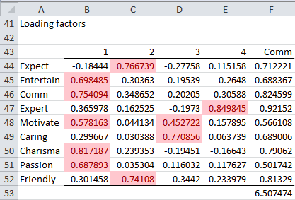
Figure 2 contains the table of loading factors from Figure 1 restricted to only the four highest common factors. Since all but the Expect loading for Factor 1 is negative, we first decide to negate all the loading factors for Factor 1. This is not a problem since the negative of a unit eigenvector is also a unit eigenvector.

Figure 2 – Loading factors and communalities for 4 factors

In addition, we recalculate the communalities for each of the variables (in column F). We can think of a communality as something like R² from regression analysis. In fact, if we perform regression analysis on the four factors, the value of R² would be 6.60747, which represents the total variance (out of 9) captured by the model (i.e. 72.3%). The communalities for each of the variables range from 50.2% for Passion to 92.2% for Expertise. Note that 72.3% of the total variance is the same percentage that we saw in Figure 1, found by dividing the sum of the eigenvalues for the highest four factors by the total variance.

In general, we would like to see that the communalities for each variable are at least .5. Variables with communalities less than .5 should be considered for removal and the analysis rerun.

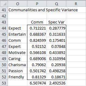
Since the variance of each variable is 1, the specific variance is simply 1 – the communality, i.e. ϕ_i = 1 – , as summarized in Figure 3. The communalities are the variances captured by the model and the specific variance are the error terms.

Figure 3 – Communalities and specific variances

As we did in Figure 9 of Principal Component Analysis, we highlight all the loading factors whose absolute value is greater than .4 (see Figure 2). We see that Entertainment, Communications, Motivation, Charisma and Passion are highly correlated with Factor 1, Motivation and Caring are highly correlated with Factor 3 and Expertise is highly correlated with Factor 4. Also, Expectation is highly positively correlated with Factor 2 while Friendly is negatively correlated with Factor 2.

Ideally, we would like to see that each variable is highly correlated with only one factor. As we can see from Figure 2, this is the case in our example, except that Motivation is correlated with both Factor 1 and 3. We will attempt to clarify the analysis by means of a rotation, as in Rotation.

References

Johnson, R. A., Wichern, D. W. (2007) Applied multivariate statistical analysis. 6th Ed. Pearson
https://mathematics.foi.hr/Applied%20Multivariate%20Statistical%20Analysis%20by%20Johnson%20and%20Wichern.pdf
Rencher, A.C., Christensen, W. F. (2012) Methods of multivariate analysis (3nd Ed). Wiley
I just got 2 factors extracted after factor analysis based on eigen value greater than 1. Is that good?
It is perfectly acceptable to have two such factors.
Charles
while conducting EFA in spss, I found 6 factors for a variable having eigenvalue greater than 1 but I just wanted to take only four factors… to do so I have to choose command “fixed number of factors to extract” and write 4 in the options box. while reporting scree plot I have 6 factors showing eigenvalues greater than 1 while in fact, I am reporting 4 factors… I just want to know it is the correct method to report results?
please answer at earliest.
I am sorry, but I don’t use SPSS and so I don’t know the answer to your question. An approach using Excel is described on this website.
Hi, used real Stats to calculate factor analysis according to the example given in this website. However, I couldn’t find a way to generate factor loadings/ loading items Table using the tool (which is shown above in figure 2). So could you please explain me how to generate the factor loading table, as without this table I don’t know how to group the variables into the factors!!
Hi Ali,
You can look at the webpage https://real-statistics.com/multivariate-statistics/factor-analysis/real-statistics-support-factor-analysis/ to see how to use the Factor Analysis data analysis tool supplied in the Real Statistics Resource Pack. You can also download the example described on the website as described on the webpage https://real-statistics.com/free-download/real-statistics-examples-workbook/