A number of methods are available to determine the factor loadings used for factor analysis. We will start by explaining the principal component method. Another commonly used method, the principal axis method, is presented in Principal Axis Method of Factor Extraction.
Using the concepts described in Basic Concepts of Factor Analysis, we describe how to carry out factor analysis via the following example.
Example
Example 1: Carry out the factor analysis for evaluating great teachers based on the data in Example 1 of Principal Component Analysis.
As we see in Example 1 of Principal Component Analysis, nine criteria are measured. Our objective is to find a set of fewer than nine factors that reasonably captures what is a great teacher. In fact, we hope to find substantially fewer than nine factors that do the job.
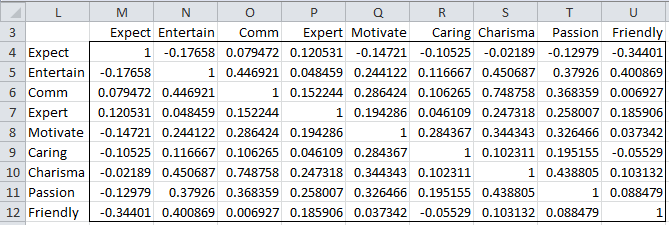
Figure 1 shows the correlation matrix for this data (repeated from Figure 4 of Principal Component Analysis).

Figure 1 – Correlation Matrix
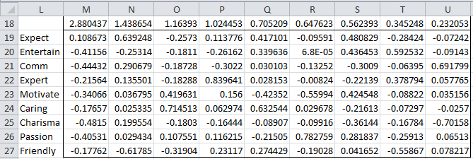
Now, Figure 2 shows the table of eigenvalues and eigenvectors for the correlation matrix (repeated from Figure 5 of Principal Component Analysis) using the Real Statistics function eigVECTSym(M4:U12).

Figure 2 – Eigenvalues and eigenvectors
Using the formula bij = cij where C1, …, Ck are the eigenvectors (range M19:U27 in Figure 2) corresponding to the eigenvalues (range M18:U18 in Figure 2) λ1 ≥ ⋯ ≥ λk, we calculate the loading factors for the nine common factors (see Figure 3).

Figure 3 – Loading factors (full model)
For example, the loading factor of the Passion variable on Factor 1 (cell B38) is given by the formula =B26*SQRT(M$18). Figure 3 also contains the communalities (range K31:K39). The communality of each variable represents the portion of that variable’s variance captured by the model. For variable xi this is . E.g., the communality of the Passion variable (cell K38) is calculated via the formula =SUMSQ(B38:J38). Since we are using the full model (where all nine common factors are present) and the variance of each variable is 1 (remember we standardized the data), it is not surprising that column K contains all ones.
Examples Workbook
Click here to download the Excel workbook with the examples described on this webpage.
Links
References
Johnson, R. A., Wichern, D. W. (2007) Applied multivariate statistical analysis. 6th Ed. Pearson
https://mathematics.foi.hr/Applied%20Multivariate%20Statistical%20Analysis%20by%20Johnson%20and%20Wichern.pdf
Rencher, A.C., Christensen, W. F. (2012) Methods of multivariate analysis (3nd Ed). Wiley
Hi Charles,
could you please explain me how could I obtain the factor correlations. It would be a square symmetric matrix of dimension mxm where m is the number of factors and diagonal 1.
Thanks for your support
Diego
Diego,
This is explained just before Figure 4 of the following webpage
https://real-statistics.com/multivariate-statistics/factor-analysis/principal-component-analysis/
by using the Real Statistics function CORR. It can also be done using a standard Excel formula or by using Excel’s Correlation data analysis tool.
Charles
Hello Charles,
How can you get the X values, using: xi=mu + L.f + e ?
Imagine you have 10 observations and 3 traits
– x would be a 10×3 matrix
– mu a 10 x 1 matrix
But L.f’s shape wouldn’t match the shapes above?…how can we get back to the original x’s values once you have decomposed the X’s?
I hope the question makes sense.
I read somewhere you had a book ready to be published? 🙂
Many thanks,
Fred
Fred,
These sort of questions are addressed at https://real-statistics.com/multivariate-statistics/factor-analysis/basic-concepts-factor-analysis/
This webpage and the other webpages on Factor Analysis show how to do this using an example.
The book is scheduled to be published in the September/October timeframe.
Charles
Hi Charles,
Regarding the first question, how to convert the original data value of X into a value of the factor Z. I understand from the tutorial, that x can be represented as a linear combination of Z but given X, how to know Z in order to proceed with the regression?
Thanks.
Adel,
If I understand your question, the Z are the factors. The calculation of the factors from the original variables is described at
https://real-statistics.com/multivariate-statistics/factor-analysis/factor-extraction/
and especially on the referenced webpage.
Charles
How to calculate multiple regression after finding factor loadings?
Lata,
You use the factor loadings to convert your original data into data about the factors (i.e. the hidden variables). Then you perform regression on the data about the factor. This assumes that the y value is not part of your factor analysis.
So if you had 100 samples about the vector X = (x1, …, x20) and then used factor analysis to find factors Z = (z1, z2, z3) you would perform regression using the data (z11, z21, z31, y1), …., (z1H, z2H, z3H, yH). Here H simply means 100.
Charles
Hi Charles,
Sorry but can you explain this answer again.
For my example I have X1, X2 and Y series.
I have the Factor Load matrix via PCA (2×2 matrix)
How do I convert X1 and X2 to Z1 and Z2 to then perform my multiple regression with Y?
Is it simply a matrix multiplication of (100 x 2) x (2 × 2) to get my new Z1 and Z2 series?
Thanks in advance.
Joey,
This is explained on the following webpage: https://real-statistics.com/multivariate-statistics/factor-analysis/factor-scores/
Charles
what are the benefits of calculating factor loadings?
Rohit,
Calculation of the factor loadings is part of a process that identifies hidden factors and how to interpret the original variables in terms of the hidden factors.
Charles
what are the usefulness of communalities in factor analysis?
The communality of each variable represents the portion of that variable’s variance captured by the model.
Charles
thanks for the explanation on how to use the tool.
from
Thomas