Basic Concepts
Suppose that random variable x has a Poisson distribution with mean λ and y has a Poisson distribution with mean μ where x and y are independent, then what is the distribution of x–y?
First, note that for m ≥ 0 and n ≥ 0
![]()
When the m < 0 or n < 0, then the correspondence pdf value is zero. Thus for k ≥ 0
![]()
![]()
If k < 0 then![]()
It turns out that![]()
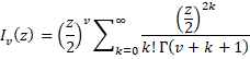
which is the pdf for the Skellam distribution where Iv(z) is the modified Bessel function of the first kind. This can be calculated in Excel by the worksheet function BESSELI(z,v).
The following formula implements the pdf for the Skellam distribution in Excel:
=EXP(-(μ+λ))*(λ/μ)^(k/2)*BESSELI(2*SQRT(μ*λ),ABS(k))
Some characteristics of the Skellam distribution are:
- Mean: λ–μ
- Variance: λ+μ
- Skewness: mean/stdev3
- Kurtosis: 3 + 1/variance
Examples
Example 1: Suppose that two soccer teams play each other and the experts estimate that the Aces will score 2.1 goals per game while the Swifts will score 1.7 goals per game.
a) What is the probability that Aces will outscore the Swifts by two goals?
b) What is the probability that the Aces will win the game?
c) What is the probability that the Swifts will win the game?
We assume that it is possible that the game ends in a tie.
We estimate the score each team will get in the game by using a Poisson distribution. Thus, to answer question (a) we use the Skellam distribution where λ = 2.3, μ = 1.7 and k = 2. The probability is 15.2% as calculated in Figure 1.
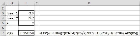
Figure 1 – Skellam distribution pdf at k = 2
The answers to questions (b) and (c) are calculated in Figure 2.
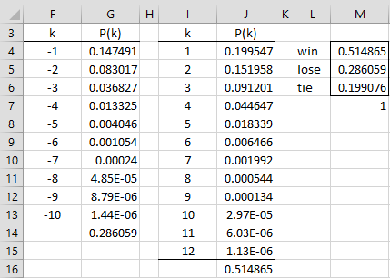
Figure 2 – Skellam distribution cdf
Questions (b) and (c)
The Aces win (question (b)) when k = 1, 2, 3, …., and so if we sum the values of P(k) for all k > 0, we will get the probability that the Aces win the game. The probability that Aces win is 51.5% as shown in column J of Figure 2. Here, cell J16 contains the formula =SUM(J4:J15). We could continue summing values of P(k) for k > 12, but it turns out that it is sufficient to sum only the first 12 entries to get 6 significant digits of accuracy.
The Swifts win when the Aces lose (question (c)), i.e. when k = -1, -2, -3, …., and so it is sufficient to sum the values of P(k) for all k < 0 (i.e. the cdf at k = -1). The probability that the Swifts win is therefore the sum of the values in column G of Figure 2, which is 28.6%, as shown in cell G14.
The probability that the game ends in a tie is therefore 100% – 51.5% – 28.6% = 19.9% (cell M6). This value can also be calculated by the formula for P(0), namely
=EXP(-(B$3+B$4))*(B$3/B$4)^(0/2)* BESSELI(2*SQRT(B$3*B$4),ABS(0))
Worksheet Function
Real Statistics Function: The Skellam distribution at x for two populations with means mean1 and mean2 can be calculated by the following Real Statistics function.
SKELLAM_DIST(x, mean1, mean2, cum) = the pdf value at x when cum = FALSE and the cdf value at x when cum = TRUE.
Thus, question (a) can be answered via the formula =SKELLAM_DIST(2,2.3,1.7,FALSE). Question (b) via the formula =SKELLAM_DIST(-1,2.3,1.7,FALSE) and question (c) via the formula =SKELLAM_DIST(-1,1.7,2.3,FALSE). Alternatively, the following Real Statistics formula addresses question (c).
=1-SKELLAM_DIST(0,2.3,1.7,TRUE)
The probability of a tie can be calculated by the Real Statistics formula =SKELLAM_DIST(0,2.3,1.7,FALSE).
Caution: The output from the SKELLAM_DIST function may be slightly in error at extreme values. For example, SKELLAM(35,20,20,TRUE) = 1.000000003, a value which is larger than 1, a result that should never happen. If the 35 is replaced by any value up to 167, the results will be similar. After 167, the values start going down, indicating a likely overflow error.
Examples Workbook
Click here to download the Excel workbook with the examples described on this webpage.
Reference
Wikipedia (2019) Skellam distribution
https://en.wikipedia.org/wiki/Skellam_distribution
A question. We already know that with the differentials I can calculate the combination of the different results in case one or the other team wins. But my question is:
How can I do so that the probabilities can be calculated: 0-0, 1-1, 2-2, 3-3….. up to 10-10, which would also be a tie but with different probabilities of occurrence?
Greetings to all for the contribution
Hello Andy,
I am sorry, but I don’t understand your question. Can you explain further?
Charles
Thank you very much for your support and contribution to the community. What I was trying to ask is that considering that the calculation of the skellam distribution works with differentials, that is, the possibility of it being:
diff: 0, 1, -1, 2, -2….n, -n
However, the probability that is ultimately interesting to predict is that of the original elements, that is, the results of each team when they face each other and their respective scores, such as:
Diff (0) = tie = 0-0, 1-1, 2-2, 3-3…
diff (1) = team A wins = 1-0, 2-1, 3-2, 4-3….
diff (-1) = team B wins = 0-1, 1-2, 2-3, 3-4….
The question is: how do I calculate from the results that we have already obtained with the skellam distribution, the different scenarios that would correspond and their probabilities for the different combinations of goals that can occur in a match?
Hello Andy,
I am still unsure wether I understand your question, but …
Skellam’s distribution is based on the difference between data from two Poisson distributions. If your scenarios use data from two Poisson distributions then you can simply use the results from this webpage.
If your original data are not based on Poisson distributions, then this approach probably won’t work.
I suggest that you state a specific example, with some real numbers, and not a range of examples, and we can try to figure out how to handle this example.
Charles
Hello, and thanks for the helpful post. However, something isn’t adding up right. I used your Excel formula to calculate a cumulative distribution function, and I’m getting sums greater than 1.0. I’m working an example with both means equal to 20 and looking at extreme tails out to +/-40.
Calculating a central probability,
P[-34<=C<=34 | λ = μ = 20] = 1.00000003566713
is the point where this goes wrong. I suspect rounding error in the BESSELI function is the cause (and a Google search confirms this). Summing over a larger range brings the error into the 7th decimal place.
I guess I either need to be less fussy about my probabilities, or figure out how to get a more accurate Bessel function. 😉
Hi Dan,
Thanks to identifying this issue.
Yes, there does seem to be an issue with roundoff error. In fact, the formula =SKELLAM(35,20,20,TRUE) produces 1.000000003 > 1. Also =SKELLAM(x,20,20,TRUE) produces 1.000000024 for x = 39 to x = 167. After x = 167 the value goes down. E.g. at x = 200, the result is .531639202, and continues decreasing from there.
For now I will give a warning that the results may be subject to randoff error at the extremes.
I appreciate your help in improving the quality of Real Statistics.
Charles
Bom dia.
Você considerou os Ases marcarem 2,1 gols por jogo, porém nos cálculos foi usado 2,3 gols por jogo (LAMBDA)
Sorry Ronaldo, but I don’t understand your comment (even after the google translation).
Charles
Your expression for the kurtosis of the Skellam distribution is wrong and should be 3 + 1/variance. That the denominator is not the mean should be obvious from the fact that the mean can be zero.
Hi Jerry,
Thanks for catching this error. I have now corrected this entry on the webpage.
I appreciate your help in improving the accuracy of the website.
Charles