Negative Binomial Distribution
Definition 1: Under the same assumptions as for the binomial distribution, let x be a discrete random variable. The probability density function (pdf) for the negative binomial distribution is the probability of getting x failures before k successes where p = the probability of success on any single trial (p and k are constants). Thus the pdf is
f(x) = C(x+k−1, x)pk(1−p)x
Worksheet Functions
Excel Functions: Excel provides the following function for the negative binomial distribution:
NEGBINOM.DIST(x, k, p, cum) = the probability of getting x failures before k successes where p = the probability of success on any single trial (i.e. the pdf of the negative binomial distribution at x) if cum = FALSE, and the probability of getting at most x failures before k successes (i.e. the corresponding cumulative negative binomial distribution at x) if cum = TRUE.
This function is not available in versions of Excel before Excel 2010. Instead, these versions of Excel use the function NEGBINOMDIST(x, k, p), which is equivalent to NEGBINOM.DIST(x, k, p, FALSE).
Real Statistics Function: Excel doesn’t provide a worksheet function for the inverse of the negative binomial distribution. Instead, you can use the following function provided by the Real Statistics Resource Pack.
NEGBINOM_INV(α, k, p) = smallest integer x such that NEGBINOM.DIST(x, k, p, TRUE) ≥ α.
Note that the maximum value of x is 1,024,000,000. A value higher than this produces an error value. This function is only available for users of Excel 2010 or later.
Properties
Key statistical properties of the negative binomial distribution are:
- Mean = k(1 – p) ⁄ p
- Variance = k(1 – p) ⁄ p2
- Skewness = (2 – p) ⁄
- Kurtosis = 6/k + p2/(k(1-p))
}")
Relation with Poisson Distribution
By algebra, the variance can also be expressed as μ(1+μ/k).
![]()
From this expression, we see that the higher the value of k the lower the variance. In fact, when k is very large, we get the assumption for the Poisson distribution, namely that the mean and the variance are equal.
Examples
Example 1: In a particularly delicate process for manufacturing a particular type of experimental silicon chip, the probability of successfully producing a marketable chip is 70%. The company needs to produce 12 marketable chips but only has the budget to manufacture 15 chips. What is the probability that they will be able to produce 12 marketable chips in at most 15 attempts?
The probability that they will make 12 marketable chips with at most 3 unacceptable chips is 29.7% as shown in cell B17 of Figure 1.
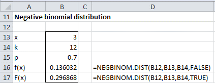
Figure 1 – Example of NEGBINOM.DIST
Example 2: How many chips described in Example 1 need to be manufactured so that the probability of getting at least 12 marketable chips is 95%?
The answer is given by the formula
=NEGBINOM_INV(.95, 12, .7) + 12
which has value 10 + 12 = 22.
Version where x and/or k are not integers
If you allow x to take non-integer values and use the gamma function where x! = Γ(x+1), then the negative binomial distribution becomes the Polya distribution with pdf for x ≥ 0
![]()
Actually, for our purposes the case where k is not an integer is more interesting. The following worksheet formulas and functions address the case where x and/or k is not an integer.
First, we note that if x is not an integer NEGBINOM.DIST truncates x to the next lower integer. The same is true if k is not an integer. Thus NEGBINOM.DIST(x, k, p, cum) = NEGBINOM.DIST(INT(x), INT(k), p, cum) when x ≥ 1 and k ≥ 1. This function returns an error value when x < 1 or k < 1.
Excel formulas
To avoid this problem, you can use the following Excel formulas instead of NEGBINOM.DIST(x, k, p, FALSE)
=EXP(GAMMALN(x+k)-GAMMALN(x+1)-GAMMALN(k)+k*LN(p)+x*LN(1-p))
=EXP(GAMMALN(x+k)-GAMMALN(x+1)-GAMMALN(k))*p^k*(1-p)^x
The formula NEGBINOM.DIST(x, k, p, TRUE) can be replaced by
=BETA.DIST(p, k, x+1, TRUE)
Where x = 0, you can replace =NEGBINOM.DIST(x, k, p, FALSE) by
=BETA.DIST(p, k, 1, TRUE)
For count values of x > 0, you can use
=BETA.DIST(p, k, x+2, TRUE)-BETA.DIST(p, k, x+1, TRUE)
Worksheet Function
The Real Statistics Resource Pack will provide the following worksheet functions:
NEGBINOM_DIST(x, k, p, cum) = the pdf of the above version of the negative binomial distribution when cum = FALSE and the cdf when cum = TRUE.
NEGBINOMX_INV(α, k, p) = smallest integer x such that NEGBINOM_DIST(x, k, p, TRUE) ≥ α.
Geometric Distribution
The geometric distribution is a special case of the negative binomial distribution, where k = 1. The pdf is
![]()
The cumulative distribution function (cdf) of the geometric distribution is
![]()
The pdf represents the probability of getting x failures before the first success. The cdf represents the probability of getting at most x failures before the first success.
Worksheet Functions
The Real Statistics Resource Pack provides the following worksheet functions:
GEOM_DIST(x, p, cum) = NEGBINOM.DIST(x, 1, p, cum)
GEOM_INV(p, pp) = NEGBINOM_INV(p, 1, pp)
Properties
The geometric distribution is memoryless. Suppose that you intend to repeat an experiment until the first success. Given that the first success has not yet occurred, the conditional probability distribution of the number of additional trials required until the first success does not depend on how many failures have already occurred. The die one throws or the coin one tosses does not have a “memory” of any previous successes or failures. The geometric distribution is the only memoryless discrete distribution that we will study.
Other key statistical properties of the geometric distribution are:
- Mean = (1 – p) ⁄ p
- Mode = 0
- Range = [0, ∞)
- Variance = (1 – p) ⁄ p2
- Skewness = (2 – p) ⁄
- Kurtosis = 6 + p2 ⁄ (1 – p)

On average, there are (1 – p) ⁄ p failures before the first success. If we include this first success, then the mean becomes 1 + (1 – p) ⁄ p, which is 1/p.
Examples
Click here to see various examples where the geometric distribution is used.
Examples Workbook
Click here to download the Excel workbook with the examples described on this webpage.
References
Wikipedia (2012) Negative binomial distribution
https://en.wikipedia.org/wiki/Negative_binomial_distribution
Forbes, C. Evans, M, Hastings, N., Peacock, B. (2011) Statistical distributions. 4th Ed, Wiley
https://www.wiley.com/en-us/Statistical+Distributions%2C+4th+Edition-p-9780470390634
Dr. Charles,
For a count data which is showing over dispersion in Poisson distribution, how to test if it follows a negative binomial distribution?
How do I calculate expected distribution frequencies and dispersion index analysis for negative binomial distribution?
I’m using the NEGBINOM_INV(p, k, pp) function but I keep getting an error.
“Compile error in hidden module: Misc”
I tried the following NEGBINOM_INV(0.5, 2, 0.25)
I’m assuming that pp = p^2.
I figured out the “Compile error in hidden module: Misc” error. Apparently, this doesn’t work on the Mac version of Excel. It worked fine on my Excel 365 version.
I am still unclear about the “pp” in the argument. Is it p^2?
MB,
pp is just the name of a variable. It is not p^2.
Charles
Charles,
What variable does pp denote?
MB
MB,
The webpage states that
NEGBINOM_INV(p, k, pp) = smallest integer x such that NEGBINOM.DIST(x, k, pp, TRUE) ≥ p.
Perhaps, it would have been clearer if I had written this as
NEGBINOM_INV(alpha, k, p) = smallest integer x such that NEGBINOM.DIST(x, k, p, TRUE) ≥ alpha.
In any case, pp is the probability of success on any one trial (just like the p in the formula for BIONOM.DIST(x,n,p,cum)).
Charles
MB,
NEGBINOM is not supported in Excel 2007 or the Mac version of Excel. This may be why you got the error message. pp is not equal to p^2.
See my response to your later comment.
Charles
“although I may indeed add a donation request sometime in the future so that I can recover some of my costs.”
When you do, please let me know at gami.nasir@gmail.com
Keep up the good work
Thanks
Gami
Gami,
Thanks for your support. I hope to decide soon, but something keeps coming up that slows down the process.
Charles
Hello Dr. Charles,
I wanted to know if there was a way to calculate 95% confidence interval from data points that follow a negative binomial distribution.
I know that it is possible to get 95% CIs using the Poisson distribution in excel using CHIINV, see this link: http://www.nwph.net/Method_Docs/User%20Guide.pdf
I would greatly appreciate any suggestions,
Angy
Hello Dr. Charles,
Is there a function in excel 2010 for the “Geometric Distribution”?
Thanks
PS: Why don’t you include a donation bottom at the end of each page?
People like me would be very happy to donate to the great work you are doing
Hello Gami,
There is no explicit geometric distribution function. Instead you need to use the formula =NEGBINOM.DIST(x,1,p,cum).
I appreciate your support. I haven’t tried to raise any money from the site, although I may indeed add a donation request sometime in the future so that I can recover some of my costs.
Charles
If NEGBINOM.DIST(x, y, p, TRUE) = the p(y) of “at most” x failures before a y success;
can I use 1-negbinom.dist(x, y, p, true) = for the p(y) of “at least” x failures before a y success ?
Pierre,
1-negbinom.dist(x, y, p, true) = the probability of at least x+1 failures before y successes.
Charles
Can you suggest me a real application of nagetive binomial distribution in reliability and survival analysis? Which are used as a life time model in reliability analysis.
With a constant failure rate and a defined number of eliminations (i.e. deaths), the expected survival rate follows the negative binomial distribution. There are lots of examples of this in healthcare, econometrics, etc. You can look at the Survival Analysis webpages on the website for some examples.
Charles