Binomial Distribution and Random Walks

We start by considering the following problem and then show how it relates to the binomial distribution.

Example 1: Suppose you start at point 0 and walk either one unit to the right or one unit to the left, where there is a 50-50 chance of either choice. Now repeat this process 100 times. What is your expected distance from the starting point?

Basic Concepts

This is a simple form of what is called a random walk problem. Define the random variables x_i as follows:

Now let d_n = your distance from the starting point after the nth trial. Thus

To solve Example 1 we need to find the expected value E[d₁₀₀]. We accomplish this by using Properties 1 and 2.

Properties

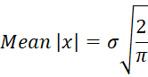
Property 1: If x ∼ N(0, σ²), then 

Proof: See proof of Property 5 of Advanced Properties of Probability Distributions.

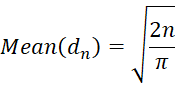
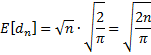
Property 2: For n sufficiently large

Proof: Let {x₁, …, x_n} be a random walk for x = .  First we note that the mean of each x_i is (.5(1) + .5(-1))/2 = 0 and the variance is ((1-0)² +(-1-0)²)/2 = 1; i.e. x_i ∼ N(0, 1). 

The random walk can therefore be considered to be a random sample from a standard normal distribution, and so by Corollary 1 of the Central Limit Theorem, for n sufficiently large, the sample mean of x is approximately normally distributed with mean 0 and standard deviation 1/. But the sample mean of x is . Thus

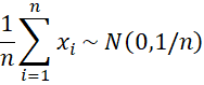
By Property 1 of Basic Characteristics of the Normal Distribution, it follows that

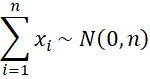
and so by Property 1

Examples

Example 1 (continued): We can now use Property 2 to complete Example 1, as follows:

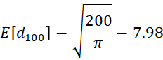
and so we see that on average your distance from the starting point is just under 8 units. Sometimes you end up to the right of the starting point and sometimes you end up to the left of the starting point (and sometimes, although far less often, you end up right back at the starting point).

Example 2: Suppose you toss a fair coin 100 times. By Property 1 of Binomial Distribution, the average number of heads is 100(.5) = 50 and the average number of tails is 50. But we know that 100 tosses won’t always result in 50 heads and 50 tails. So on average how many more or fewer heads are there than the average of 50?

It is easy to see that the answer to this question is the average value of |# of heads – 50|. But what is this value?

If we view getting heads as going right and getting tails as going left in our random walk problem, we see that the solution to this example is also E[d₁₀₀]. In general, the average number of heads after n tosses is n/2 and so

the average value of |# of heads after n tosses – n/2| = E[d_n]

Since

we see that the answer to Example 2 is again just under 8. In fact, this means that not only is it not necessarily the case that heads and tails break 50-50 in 100 tosses but on average heads are 8 units away from 50, i.e. on average, heads and tails break 58-42 (although not necessarily is the 58 for heads).

Observation

Note that for any a and b, |a| < b is equivalent to –a < b < a. Since, as we have seen above,  ~ N(0,), it follows that the probability that d_n = || < k for any value of k is NORM.DIST(k, 0, SQRT(n), TRUE) – NORM.DIST(-k, 0, SQRT(n), TRUE) = 2*NORM.DIST(k, 0, SQRT(n), TRUE)–1.

For example, P(d₁₀₀ < 7) = .758 – .242 = .516.

References

Hoel, P. (1962) Introduction to mathematical statistics, 3^rd Ed. John Wiley and Sons

Tijms, H. (2007) Understanding probability: chance rules in everyday life (2^nd ed.). Cambridge: Cambridge University Press.

http://scholar.google.it/scholar_url?url=http://personal.vu.nl/h.c.tijms/SampleUP.pdf&hl=en&sa=X&ei=R1HXYPKlOM6Fy9YPgKCj4Ak&scisig=AAGBfm2n1zaissHo6sIEY1rVxlZHprY2Mg&nossl=1&oi=scholarr