Basic Concepts
The (Beta) PERT distribution can be useful when you only have limited information about a distribution, provided you can estimate the upper and lower bounds, as well as the most likely value. In fact, the distribution is based on the following three parameter values:
- a = minimum value
- b = mode
- c = maximum value
This distribution can be used to calculate the likely time to complete a project or project step (e.g. as described in a PERT diagram) based on an optimistic, pessimistic and most likely time frame.
It is defined so that the mean and standard deviation take the following values:
![]()
The cdf for PERT distribution is equal to BETA.DIST(x, α, β, TRUE, a, b) or BETA.DIST(z, α, β, TRUE) where
![]()
and the pdf for PERT distribution is equal to BETA.DIST(x, α, β, FALSE, a, b).
Key statistical properties of the PERT distribution are shown in Figure 1.

Figure 1 – Statistical properties of the PERT distribution
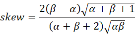
We can also calculate skewness by the formula
Worksheet Functions
Real Statistics Functions: Excel provides the following functions:
PERT_DIST(x, a, b, c, cum) = the pdf of the PERT function f(x) when cum = FALSE and the corresponding cumulative distribution function F(x) when cum = TRUE.
PERT_INV(p, a, b, c) = x such that PERT_DIST(x, a, b, c, TRUE) = p; i.e. the inverse of the cdf of PERT distribution.
You can also obtain the pdf, cdf, and inverse function of the PERT distribution from the beta distribution. In particular, we have the following equivalent Excel formulas.
PERT_DIST(x, a, b, c, cum) = BETA.DIST(x, α, β, cum, a, c)
PERT_INV(p, a, b, c) = BETA.INV(p, α, β, a, c)
where α and β are defined from a, b, and c as described previously.
Examples
Example 1: Create a plot of the PERT distribution for data with a min of 1, max of 9, and mode of 6. Also, what is the mean and standard deviation of this distribution?
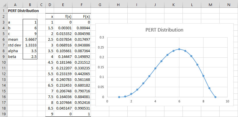
Figure 1 – PERT distribution
From Figure 1, we see that the mean is 5 2/3 (cell B6) and the standard deviation is 1 1/3 (cell B7), as calculated respectively by the formulas =(B3+4*B4+B5)/6 and =(B5-B3)/6, respectively.
The values for alpha (cell B8) and beta (cell B9) are 3.5 and 2.5, as calculated by the formulas =4*(B4-B3)/(B5-B3)+1 and =4*(B5-B4)/(B5-B3)+1.
We create a plot of the distribution from 1 to 9 in .5 increments based on the values in range D3:E19. This is done by placing the formula
=BETA.DIST(P3,$B$8,$B$9,FALSE,$B$3,$B$5)
in cell E3, highlighting the range E3:E19 and pressing Ctrl-D. Alternatively, we could place the following Real Statistics formula in cell E3.
=PERT_DIST(D3,$B$3,$B$4,$B$5,FALSE)
The chart is shown on the right side of Figure 1.
We can also calculate the cumulative distribution function cdf values by placing either of the following formulas
=BETA.DIST(P3,$B$8,$B$9,TRUE,$B$3,$B$5)
=PERT_DIST(D3,$B$3,$B$4,$B$5,TRUE)
in cell F3, highlighting the range F3:F19 and pressing Ctrl-D.
Observation: We can see from Figure 1 that the median of the distribution occurs somewhere between x = 5.5 and x = 6.0. In fact, with a little experimentation, we see that the correct value occurs at about x = 5.74524. This can be verified using the formula =PERT_INV(B3,B4,B5).
Examples Workbook
Click here to download the Excel workbook with the examples described on this webpage.
References
Wikipedia (2019) PERT distribution
https://en.wikipedia.org/wiki/PERT_distribution
Wikipedia (2019) Beta distribution
https://en.wikipedia.org/wiki/Beta_distribution
Broadleaf (2014) Beta-PERT origins
http://broadleaf.com.au/resource-material/beta-pert-origins/
VOSE Software (2017) PERT distribution
https://riskwiki.vosesoftware.com/PERTdistribution.php
Thank you very much for this clarification.
I use the Beta.dist function in Excel to estimate the PERT distribution by calculating alpha and beta as you describe. The formula for alpha and beta both have “4” in the equations. Is this the same “4” as in the “definition” of the mean?
Some Beat distribution tools refer to a parameter called “lambda”. Is this the same as the “4”?
Hello Kim,
I believe that you are correct that the “4” in the definition of alpha and beta becomes the “4” in the mean.
I am not familiar with lambda, but in looking at https://www.riskamp.com/beta-pert it does appear that “lambda” is the same as “4”.
Charles
I wonder what happened to my recent post questions on December 12-13?
Thanks,
You can view your comment now. I will respond shortly.
Charles
Dear Charles,
I have another question to ask of you and validate some of my calculations regarding the Variance formula of PERT distribution (c-a)^2/36, which I often doubt? Using calculus integration of the PDF of PERT distribution for any given parameters (α, β, a, b, c), I find the value of Integral [ Integral(a to c) of ( u – E(u) )^2 * f_PERT.pdf(u) du ] equals to ===>
(αβ/7)*(c-a)^2/36 rather than (c-a)^2/36. Any feed back is appreciated on my findings.
Thank you!
Fixing a typo in the formula ** [(αβ/7)*(c-a)^2/36] ** , I wish I could just paste images here :)!
Nazih.
Hello Nazih,
I just used the new Real Statistics INTEGRAL function to check your conclusion and I found that it holds up.
It does seem like the variance is (αβ/7)*(c-a)^2/36. I just checked a few sources and they all say (c-a)^2/36.
It is not clear to me why they are all giving the wrong result (or alternatively, why we think your result is correct).
Charles
I just checked and if you derive the variance from the beta distribution you get (αβ/7)*(c-a)^2/36, as you stated.
I wonder why all the references leave out the (αβ/7) factor.
Charles
Is it true to assume for PERT Distribution above that (alpha + beta) is always equal to 6 ?!
Yes. If you add the expressions for alpha and beta you will get 6. Nice observation.
Charles
Great page, thank you. I ran some numbers using your formulas and it occurred to me that if the intention is for the BetaPERT distribution to have a range of ~6 standard deviations (as originally intended by the creators), the shape parameters must add up to 8, not 6. For example, B(4, 4) has the Range [0, 1] and a Standard Deviation of exactly 1/6, which is why the 68-95-99 Rule holds true. As the distribution skews to B(3, 5) or even more towards B(2, 6), the σ = R/6 relationship begins to break down, but it remains reasonably approximate for most moderately skewed distributions.
In contrast, B(3, 3) has a σ =R/5.3, which is much more spread out, and it deteriorates more rapidly as the distribution skews towards B(2, 4). This is less consistent with the creators original intention of σ = R/6 and of course it means the 68-95-99 Rule does not work nearly as well.
You should consult with someone that has better theoretical knowledge of the math, but I believe adjusting the shape parameter formulas to =6*(B4-B3)/(B5-B3)+1 and =6*(B5-B4)/(B5-B3)+1 would adjust the sum of the shape parameters to be fixed at 8, which should also make your σ = ~R/6.
Referring to Figure 1, the distribution ranges from 1 to 9, a range of 9-1 = 8. If this range spreads 6 standard deviations, then the standard deviation should be 8/6 = 1.333, which is indeed the standard deviation, as shown in cell B7. I don’t understand what the problem is.
Charles
In that case, then for simplicity, Skewness and Kurtosis should be rewritten as follows:
Skewness = 2(β – α)/sqrt(7αβ)
Kurtosis = 7(α – β)^2/12αβ – 1/9
I am not sure how you arrived at these values. I got
skewness = (β – α)*sqrt(7/αβ)/4
kurtosis = 7(β – α)^2/(12αβ) – 2/3 = (4/3)*skewness^2 – 2/3
Perhaps, you are correct and I made an algebra mistake, but if so, I can’t find the mistake.
In any case, I like the way you are trying to simplify the expressions
Charles
You are correct Dr. Zaiontz (somehow my algebra was off), with (α + β = 6 ), then ⇉
skewness = 7(β – α) / 4*sqrt(7αβ) ⟺ (β – α)*sqrt(7/αβ)/4.
kurtosis = 7(α – β)^2/(12αβ) – 2/3.
Also, the PERT distribution itself can be rewritten in terms of either just α (or just β).
By the way, I love the work you have done here. Although I use R, however there are times I find myself on your website. Thank you!