Real Statistics Support for Two Factor Anova

Functions using Excel input format

On this webpage, we show how to conduct Two Factor ANOVA for balanced models using capabilities found in the Real Statistics Resource Pack.

Real Statistics Excel Functions: The Real Statistics Resource Pack supplies the following functions. Here R1 contains the sample data and r is the number of rows for the A factor.

SSWF(R1, r) = SSW	dfWF(R1, r) = dfW	MSWF(R1, r) = MSW
SSRow(R1, r) = SSA	dfRow(R1, r) = dfA	MSRow(R1, r) = MSA
SSCol(R1, r) = SSB	dfCol(R1, r) = dfB	MSCol(R1, r) = MSB
SSInt(R1, r) = SSAB	dfInt(R1, r) = dfAB	MSInt(R1, r) = MSAB
SSTot(R1, r) = SST	dfTot(R1, r) = dfT	MSTot(R1, r) = MST

The second argument for the column and interaction functions is optional and can be dropped.

ANOVARow(R1, r) = MSA/MSW	ATestRow(R1, r) = p-value for A factor
ANOVACol(R1, r) = MSB/MSW	ATestCol(R1, r) = p-value for B factor
ANOVAInt(R1, r) = MSAB/MSW	ATestCol(R1, r) = p-value for AB factor

Observation: For example, referring to Example 1 of Two Factor ANOVA with Replication (esp. Figure 2 on that webpage), MSRow(B5:E19, 5) = 4391.45, which is the same result obtained in cell J30 of Figure 3 of that webpage. Similarly, ATESTInt(B5:E9, 5) = 0.04556, which is the same as cell L32 of Figure 3 on that webpage.

Observation: These functions also support Two Factor ANOVA without Replication by setting the value of r to 1.

Data analysis tools based on Excel input format

Real Statistics Data Analysis Tool:  The Real Statistics Resource Pack provides the Two Factor ANOVA data analysis tool, which we demonstrate in the following example.

Example 1: Perform the analysis of Example 1 of Two Factor ANOVA with Replication using the Real Statistics Two Factor ANOVA data analysis tool.

Click on cell G1 (where the output will start), press Ctrl-m and double click on the Analysis of Variance option (or click on the Anova tab if using the multipage interface). The dialog box shown in Figure 1 will appear.

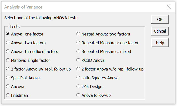
Figure 1 – Dialog box for Analysis of Variance

Choose the Anova: two factors option and click on the OK button. The dialog box shown in Figure 2 will now appear.

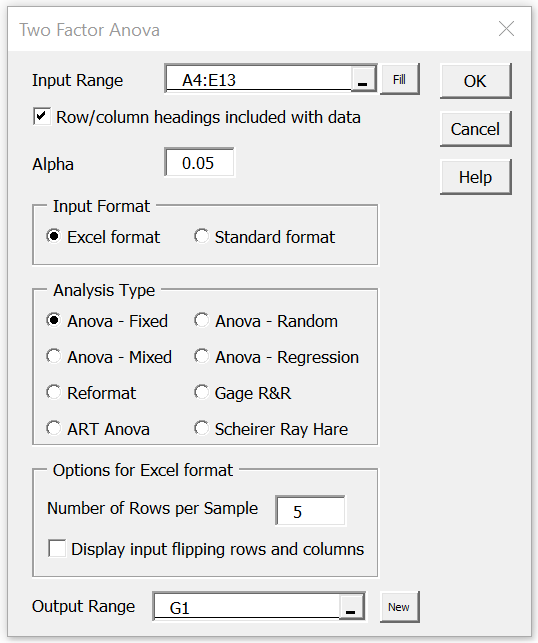
Figure 2 – Dialog box for Two Factor Anova

Enter A4:E19 in the Input Range, click on Column/row headings included with data, select Excel format as the Input Format and select the ANOVA as the Analysis Type. Next, insert 5 in the Number of Rows per Sample field and click on the OK button. The output is shown in Figure 3.

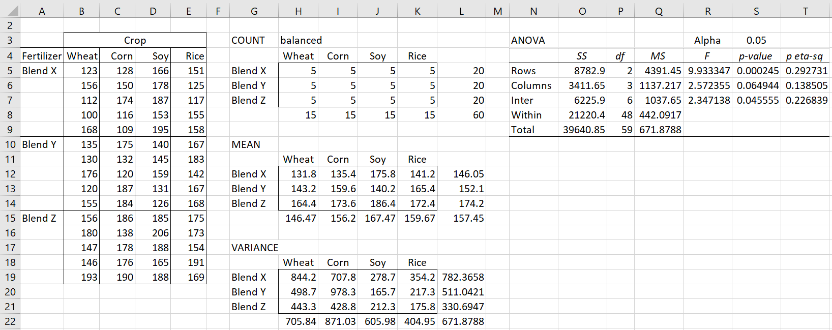
Figure 3 – Two Factor ANOVA data analysis

Three tables of descriptive statistics, as well as the ANOVA results, are produced. Note that the Interaction table (range G11:L15) is as Figure 3 of Two Factor ANOVA with Replication, and can be used to create the charts shown in Figure 4 of that webpage.

Observation: If the Number of Rows per Sample field is set to 1, then two-factor ANOVA without replication is used.

Observation: The data analysis tool also provides the option to exchange the rows and columns of the input range. This will be useful when performing follow-up analyses (see for example Contrasts for Two Factor Anova).

To do this for the data in Example 1 check the Display input flipping rows and columns option shown in Figure 2. The output is shown in Figure 4.

Figure 4 – Exchanging rows and columns in input data range

In addition to the analysis of the main effects (Blend and Crop in the above example), The Real Statistics Two Factor ANOVA Follow-up data analysis tool can be used for a variety of follow-up tests, including contrasts and Tukey’s HSD, as well as simple effects, as shown in the next example.

Example 2: Show the analysis of the Crops simple effects for the data in Figure 3.

This is done by pressing Ctrl-m, double-clicking on the Analysis of Variance option (or clicking on the Anova tab if using the Multipage interface) and selecting the Two Factor ANOVA Follow-up option (as shown in Figure 1). After pressing the OK button, fill in the dialog box that appears as shown in Figure 5.

Figure 5 – Dialog box for Two Factor ANOVA Follow-up tests

Note that you need to enter the group means range (as shown in range H12:K14 of Figure 3) in the Input Range field. Upon pressing the OK button, the output is as shown in Figure 6.

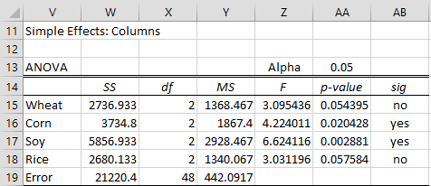
Figure 6 – Crops Simple Effects

Stacked input format

Two input formats are supported by the data analysis tool. The Excel format is the one used by Excel, as described in Figure 3 The data analysis tool also supports what we will call the standard format, also called stacked format.

This format consists of a range with three columns. The first column contains the row group names (blends in the above example), the second column contains the column group names (crops in the above example) and the third column contains the corresponding scores (yield in the above example). The rows can be listed in any order.

Example 3: Perform an analysis of variance for the data in range A3:C27 of Figure 7.

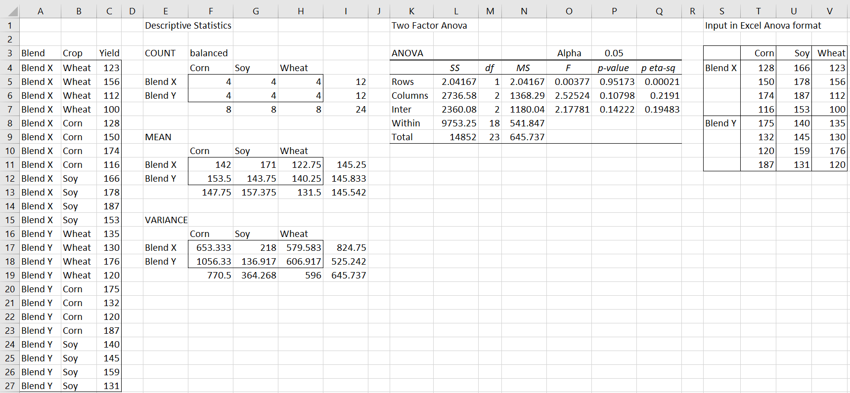
Figure 7 – Two Factor ANOVA on data in standard format

To do this, click on cell E1 (where the output will start), enter Ctrl-m and select the Two Factor ANOVA option from the menu that appears. When the dialog box in Figure 1 appears, enter A3:C27 in the Input Range, click on Column/row headings included with data, select Standard format as the Input Format, select ANOVA as the Analysis Type and click on the OK button. The output is shown in Figure 7.

The output is similar to that obtained when the Excel input format is used and includes descriptive statistics tables and the ANOVA results. In addition, the input data is converted into the Excel format (range S3:V11). This will be useful when follow-up tests are conducted.

Real Statistics Functions: The Real Statistics Resource Pack contains the following array functions for converting between Two Factor Anova Excel format and standard format.

StdAnova2(R1):  takes the data in R1 which is in standard format (without column headings) and outputs an array with the same data in Two Factor Anova format (with row/column headings).

Anova2Std(R1, r): takes the data in R1 which is in Two Factor Anova format (including row/column headings) with r rows per group and outputs an array with the same data in standard format (without column headings).

Observation: Referring to Figure 4, note that =StdAnova2(A4:C27) generates the output in range S3:V11 and =Anova2Std(S3:V11,4) generates output similar to that in range A4:C27, but in sorted order.

Observation: The Two Factor Anova data analysis tool also supports the case of two-factor ANOVA without replication by setting Number of Rows per Sample to 1. The various supplemental functions also support two-factor ANOVA without replication by setting r = 1.

Observation: As we have seen above, when the input data is in standard format the Two Factor Anova data analysis tool will automatically convert the data into Excel format when the Anova analysis option is chosen. Similarly, as can be seen in Unbalanced Factorial ANOVA, when the input data is in Excel format the Two Factor Anova data analysis tool will automatically convert the data into standard format when the Regression analysis option is chosen.

Observation: In all the examples given the group samples have the same number of elements (balanced model). In Unbalanced Factorial ANOVA we show how to use the Regression option of Two Factor Anova data analysis tool to analyze unbalanced models.

Real Statistics Functions: The Real Statistics Resource Pack also supports the following functions where the data in R1 is in standard (stacked) format.

SSRowStd(R1) = SSA	SSColStd(R1) = SSB	SSIntStd(R1) = SSAB
SSWFStd(R1) = SSW	SSTotStd(R1, 3) = SST	dfWFStd(R1) = dfW
dfRowStd(R1) = dfA	dfColStd(R1) = dfB	dfIntStd(R1) = dfAB