Estimating HMM parameters with known hidden states and observations
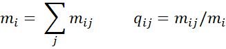
When both the sequence of hidden states (or multiple such sequences) is known, as well as the corresponding observations, we can use the approach described in Estimating Markov Chain Parameters to estimate the HMM parameters. The transition matrix and distribution array are estimated from the hidden states as described in Estimating Markov Chain Parameters. We estimate the values in the emission matrix as follows, where mij = the number of times state i maps to observation j.
Worksheet Function
The Real Statistics Resource Pack provides the following function where Rs is an n × h array containing the hidden states generated by h runs of an HMM, each of length n, and Ro is an n × h array containing the corresponding observations.
HMM_Params(Rs, Ro, k, m): returns a k × k+m+1 array, where the leftmost k × k+1 array is the estimated transition matrix + distribution array, and the rightmost k × m array is the estimated emission matrix.
Here, k defaults to the largest element in Rs and m defaults to the largest element in Ro.
Example
Example 1: Suppose 10 runs of a Markov process of length 20 result in the hidden states shown in range H2:Q26 of Figure 1 and the observations shown in range S2:AB26. Find the most likely transition matrix, distribution vector, and emission matrix.
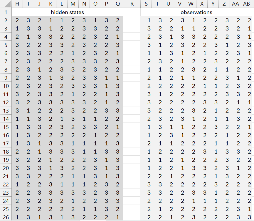
Figure 1 – HMM states and observations
Using the formula =HMM_Params(H2:Q26, S2:AB26), we obtain the output shown in Figure 2.
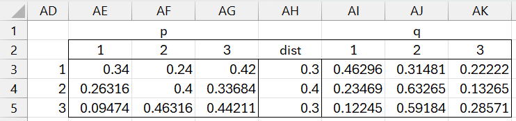
Figure 2 – Estimated HMM parameters
Iterative Viterbi Approach
Of course, the limitation with the above approach is that we usually don’t know the hidden states, only the observations. We can, however, use the Viterbi algorithm to estimate the hidden states from the observations (based on some initial estimate of the HMM parameters). Using the observations and hidden state sequences, we can generate a new, hopefully improved, version of the HMM parameters. We can continue in this fashion until convergence. Here, convergence occurs when the sequence(s) of hidden states repeats.
Example 2: Generate the HMM parameters for the observations in Example 1 (repeated in range J3:S11 of Figure 3), based on the initial guesses of the HMM parameters shown in range B2:H4.
We obtain the iterations shown in Figure 3. First, we generate the hidden states shown in range U2:AD11 using the formula =HMM_ViterbiX($B2:$D4,$E2:$E4,$F2:$H4,J2:S11). We next create a new version of the HMM parameters, as shown in range B14:H16, by using the formula =HMM_Params(U2:AD11,J2:S11).
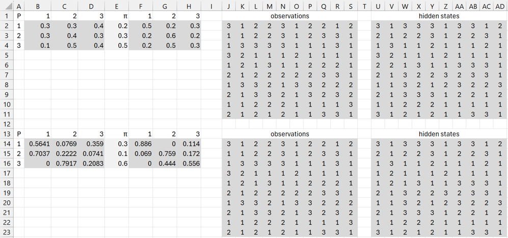
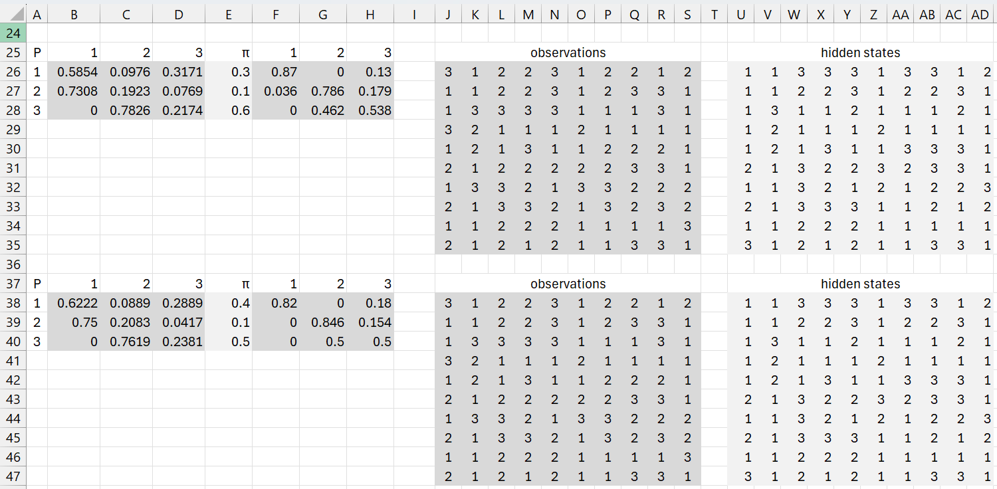
Figure 3 – Iterative approach
We repeat this process a couple of more times, as shown in Figure 3. The next iteration is identical to the last one shown in Figure 3, and so we have convergence.
Worksheet Function
The Real Statistics Resource Pack provides the following function where the arguments are the same as for HMM_BaumX, except that no precision argument is used.
HMM_ParamsX(Rp, Rd, Rq, Ro, iter): returns a k × k+m+2 array with the results of the iterative algorithm described above in the same format as HMM_BaumX (see Baum-Welch Worksheet Functions), except that no precision value is returned.
Note that the formula =HMM_ParamsX(B2:D4,E2:E4,F2:H4,J2:S11) produces the output shown in range B38:H40 of Figure 3, except that the number of iterations until convergence, namely 4, would appear in cell I38.
Initialization of the Baum-Welch algorithm
The Baum-Welch algorithm is highly dependent on the initial HMM parameter values. Since this algorithm finds a local maximum, different initial values are likely to produce different HMM matrices upon convergence. Thus, it is helpful to set the initial values as close as possible to the expected final HMM parameters.
Example 3: Redo Example 2 of Baum-Welch Worksheet Functions using the output from Example 2 to initialize the HMM parameters.
The results are shown in Figure 4. Here, the initial HMM parameters, shown in range B2:H4, are copied from range B38:H40 of Figure 3. Using the formula =HMM_BaumX(B2:D4,E2:E4,F2:H4,J2:S11,1000), we obtain the results shown in range B14:I16, which is hopefully a better estimate than the one shown in Figure 5 of Baum-Welch Worksheet Functions.
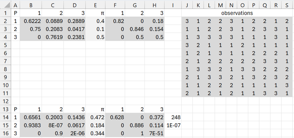
Figure 4 – Baum-Welch with Initialization
Links
Examples Workbook
Click here to download the Excel workbook with the examples described on this webpage.
References
Wikipedia (2026) Hidden Markov model
https://en.wikipedia.org/wiki/Hidden_Markov_model
Jurafsky, D., Martin, J. H. (2026) Hidden Markov models
https://web.stanford.edu/~jurafsky/slp3/A.pdf
Bouman, C. A. (2006) Markov chains and Hidden Markov models
https://engineering.purdue.edu/~bouman/ece641/previous/fall06/notes/pdf/MC-HMMs.pdf