Objective
Our goal is to find the sequence of hidden states that is most likely to generate a given sequence of observations.
We do this using Viterbi’s algorithm.
Viterbi’s algorithm
Viterbi’s algorithm finds the most likely path that ends in state s at time i and generates observations z1, …, zi.
For any sequence of states x1:i = x1, …, xi and any state s, define

We now define

We can calculate the δi(s) iteratively, as follows

Also define

We calculate ηi(s) iteratively as


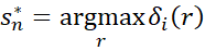
For the terminal time n, define
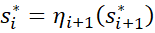
Thus, the optimum path is s1*, …, sn* where for all i < n
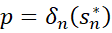
The joint probability of the most likely path is
Example
Example 1: Use Viterbi’s algorithm to find the most likely sequence of states that generates the observations shown in range H3:H12 of Figure 1 for the HMM described on the left side of the figure.
The results are also shown in Figure 1.
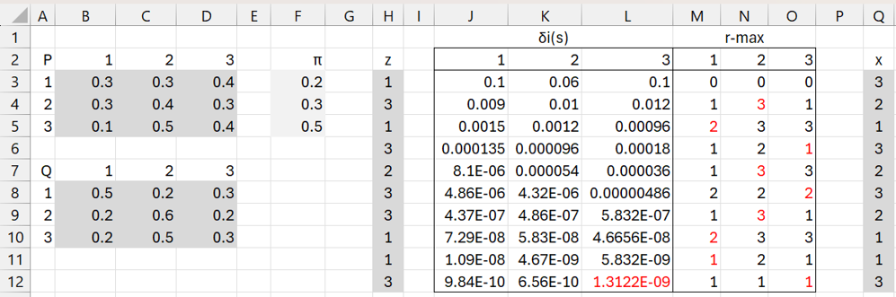
Figure 1 – Viterbi’s algorithm
Manual calculations
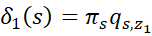
We show how to obtain the first two rows on the right side of Figure 1. For row 1, we use the formula
δ1(s) = πsqs,z1
where z1 = 1.
δ1(1) = π1q11 = .2(.5) = .10
δ1(2) = π2q21 = .3(.2) = .06
δ1(3) = π3q31 = .5(.2) = .10
We also place zeros in cells M3, N3, and O3.
For row 2, we use the formula
δ2(s) = qs,z2 ⋅ max(δ1(r)⋅prs: r in S)
where z2 = 3. Thus, for each s, we calculate δ1(r)prs for r = 1, 2, 3. For s = 1, we get
δ2(1)p11 = .1(.3) = .03
δ2(2)p21 = .06(.3) = .018
δ2(3)p31 = .1(.1) = .01
Since .03 is the largest of these values, we place r = 1 in cell M4, and multiply .03 by qs,z2. Since qs,z2 = q13 = .3, we obtain
δ2(1) = .03(.3) = .009
which we place in cell J4. We calculate δ2(2) similarly.
δ2(1)p12 = .1(.3) = .03
δ2(2)p22 = .06(.4) = .024
δ2(3)p32 = .1(.5) = .05
Since .05 is the largest of these values, we place r = 3 in cell N4, and multiply .05 by qs,z3. Since qs,z2= q23 = .2, we obtain
δ2(2) = .05(.2) = .01
which we place in cell K4. We next calculate δ2(3).
δ2(1)p13 = .1(.4) = .04
δ2(2)p23 = .06(.3) = .018
δ2(3)p33 = .1(.4) = .04
Since .04 is the largest of these values, we place r = 1 (or 3) in cell O4, and multiply .04 by qs,z3. Since qs,z3 = q33 = .3, we obtain
δ2(3) = .04(.3) = .012
which we place in cell L4.
We continue in this manner to obtain all the other values in Figure 1. We can also use Excel formulas, as follows.
Using Excel formulas
Place the formula =TRANSPOSE(F3:F5*INDEX(B8:D10,,H3)) in range J3:L3 and zeros in M3:O3.
Next, place
=MAX($J3:$L3*TRANSPOSE(INDEX($B$3:$D$5,,J$2)))*INDEX($B$8:$D$10,J$2,$H4)
in cell M4, highlight range J4:L12, and press Ctrl-R and Ctrl-D.
Finally, place the Real Statistics formula
=INDEX_MAX(INDEX($B$3:$D$5,,J$2)*TRANSPOSE($J3:$L3))
in cell M4, highlight range M4:O12, and press Ctrl-R and Ctrl-D.
The joint probability of obtaining the best path is the largest value for δ10(s), since n = 10. For Example 1, this is 1.31E-09, which occurs in cell L11 where s = 3.
State sequence
Thus
s10* = 3
Since the 3rd element in range M12:O12 is 1, it follows that
s9* = 1
Since the 1st element in range M11:O11 is 1, it follows that
s8* = 1
Backtracking in this way, we see that the most likely state sequence is
3213232113
as highlighted in red in Figure 1, and duplicated in column Q.
Real Statistics Support
Click here to learn about Excel worksheet functions provided by the Real Statistics Resource Pack in support of Viterbi’s algorithm. Includes additional examples.
Links
Examples Workbook
Click here to download the Excel workbook with the examples described on this webpage.
References
Wikipedia (2026) Hidden Markov model
https://en.wikipedia.org/wiki/Hidden_Markov_model
Jurafsky, D., Martin, J. H. (2026) Hidden Markov models
https://web.stanford.edu/~jurafsky/slp3/A.pdf
Frazzoli, E. (2010) Intro to Hidden Markov Models
https://ocw.mit.edu/courses/16-410-principles-of-autonomy-and-decision-making-fall-2010/55e488318190f148c4ed211e2c96bada_MIT16_410F10_lec20.pdf